Download Code
In this tutorial, we will demonstrate how to design a LQR controller in order to stabilize the following linear coupled (hybrid) PDE-ODE system:
Similar systems may appear in the modelling of a variety physical phenomena, such as the melting of ice in a body of water [1] or fluid-structure interaction [2]. This particular system may be seen as a simplification of the well known one-phase Stefan problem. The stabilization and control of the former has been investigated in recent works by Krstic et al. (see [1] for example). The relationship between the considered system and the Stefan problem, as well as the control of the latter will be considered in a future tutorial.
When no forces are applied, a feature of the governing parabolic PDE is its possibility of generating unstable dynamics as $t \rightarrow \infty$. This phenomenon is due to the fact that the sign of the eigenvalues of the governing elliptic differential operator depends on the magnitude of the constant $\beta$. More precisely, as the differential operator has eigenvalues of the form $\mu_k = \beta - \lambda_k$, where $\lambda_k$ are the eigenvalues of the Dirichlet laplacian, taking $\beta > \lambda_1$ (the biggest among the $\lambda_k$) would yield such a result. We will thence implement a LQR optimal control strategy in order to stabilize the system.
We first need to reduce the PDE-ODE system to a finite dimensional system of the form
where $A$ and $B$ are matrices, and
is the finite dimensional state vector.
We fix the parameters as follows: $T=1$, $\alpha=1$ and $\beta = 10$:
clc; clear;
T = 1;
nT = 100; nX = 20;
dt = T/nT; dx = 1/(nX+1);
x = linspace(0,1,nX+2);
Dir0 = 1; Dir1 = 0;
alpha = 1; beta = 10;
We begin the code by discretizing in space the parabolic PDE; this is done by finite differences:
Id = eye(nX);
Lapl = -2*Id + diag(ones(nX-1,1),-1) + diag(ones(nX-1,1),1);
A0 = alpha*1/dx^2*Lapl + beta*Id;
In fact, the finite difference discretization of the Dirichlet laplacian may also be done using the MATLAB routine delsq. We proceed similarly for the term $y_x(1,t)$ in the ODE, and assemble the complete matrix $A$:
A = zeros(nX+1,nX+1); A(2:nX+1,2:nX+1) = A0; A(1,2)=-1/dx;
The control matrix B is constructed as follows:
b = zeros(nX,1); b(1,1) = alpha*Dir0/dx^2; b(nX,1) = alpha*Dir1/dx^2;
B = zeros(nX+1,1);
B(1,1) = Dir0/dx;
B(2:nX+1,1) = b;
We may now proceed with the optimal control strategy. For a continuous time linear system generated by the matrices $(A,B)$ and an infinite time horizon cost functional defined as
the feedback control law that minimizes the value of the cost is $u = -Kz$, where $K = R^{-1}B*P$ and $P$ is found by solving the continuous time algebraic Ricatti equation
We check whether the constructed matrices fit in the framework of LQR. Namely, we first verify that the couple $(A, BB*)$ is stabilizable. This is done by checking if $\text{rank}[\lambda I - A, B] = d$ for any $\lambda \in \sigma(A)\cap \mathbb{R}_+$, where $d$ is the dimension of the state space.
eigs = eig(A);
for iter=1:nX+1
    if real(eigs(iter))>=0
        M = zeros(nX+1,2*(nX+1));
        M(:,1:nX+1) = eigs(iter)*eye(nX+1)-A; M(:,nX+2:2*(nX+1)) = B*(B');
        r_ = rank(M);
        stabilizable = (r_ == nX+1);
    end
end
Secondly, we check that the eigenvalues of the associated Hamiltonian matrix do not lie on the imaginary axis.
R = 1; Q = eye(nX+1);
H = blkdiag(A, -A');
H(nX+2: 2*(nX+1), 1:nX+1) = -Q; H(1:nX+1, nX+2: 2*(nX+1)) = -B*(B');
eigH = real(eig(H));
nb_im_eig = sum(eigH == 0);
Finally, we check if the pair $(Q, A)$ is detectable; the variable not_det should equal $0$ after the loop.
not_det = 0;
for iter_=1:nX+1
    if real(eigs(iter_))>=0
        M_ = zeros(2*(nX+1), nX+1);
        M_(1:nX+1, :) = Q; M_(nX+2:(nX+1)*2, :) = eigs(iter_)*eye(nX+1)-A;
        r_ = rank(M_);
        if (r_ ~= nX+1)
            not_det = not_det + 1;
        end
    end
end
We are now in a position to construct the LQR feedback control by solving the algebraic Ricatti equation. This is done by using the MATLAB Control Toolbox routine care:
[ricsol, cleig, K, report] = care(A, B, Q, R);
f_ctr = @(z) -K*z;
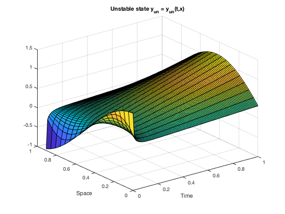
We now compare the uncontrolled (thence unstable) dynamics with the dynamics stabilized by the LQR feedback control. As initial datum for both systems, we pick $u_0(x) = \cos(\pi*x)$ and $s_0 = 0.1$.
x_int = x(1:nX);
y0 = cos(x_int*pi)';
z0 = zeros(nX+1,1); z0(1,1) = 0.1; z0(2:nX+1,1) = y0;
The free system is solved with the Dirichlet boundary condition $u(0,t) = 0.15$:
f1 = @(t,v) A*v + B*0.15;
[t1, z_free] = ode45(f1, linspace(0,T,nT), z0);
[X1,Y1] = meshgrid(t1,x_int);
surf(X1, Y1, z_free(:,2:nX+1)');
xlabel('Time');
ylabel('Space');
title('Unstable state y_{un} = y_{un}(t,x)')
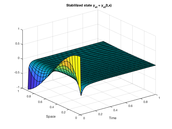
Now we solve and visualize the controlled problem:
f2 = @(t,z) A*z + B*f_ctr(z);
[t2, z_ctr] = ode45(f2, linspace(0,T,nT), z0);
figure;
[X2,Y2] = meshgrid(t2,x_int);
surf(X2, Y2, z_ctr(:,2:nX+1)');
xlabel('Time');
ylabel('Space');
title('Stablilized state y_{st} = y_{st}(t,x)')
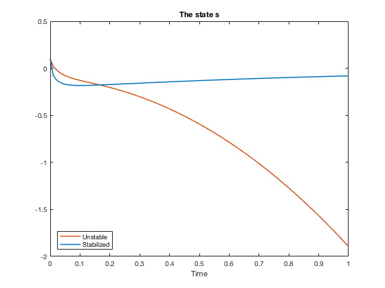
We also plot the corresponding solutions to the ODE:
figure;
plot(t1, z_free(:,1), 'Color', [0.8500, 0.3250, 0.0980], 'LineWidth', 1.5);
hold on;
plot(t2, z_ctr(:,1), 'Color', [0, 0.4470, 0.7410], 'LineWidth', 1.5);
legend('Unstable', 'Stabilized', 'Location', 'SouthWest');
xlabel('Time')
title('The state s')
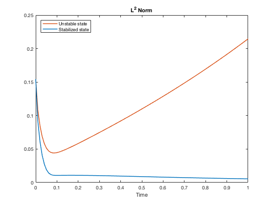
As a final test of our results, we compare the $L^2(0,1)$-norms of both the controlled and uncontrolled state with respect to time.
norm_free = 1/nX*sum(z_free.^2,2).^0.5;
norm_ctr = 1/nX*sum(z_ctr.^2,2).^0.5;
figure;
plot(t1, norm_free, 'Color', [0.8500, 0.3250, 0.0980], 'LineWidth', 1.5);
hold on;
plot(t2, norm_ctr, 'Color', [0, 0.4470, 0.7410], 'LineWidth', 1.5);
legend('Unstable state', 'Stabilized state', 'Location', 'NorthWest');
xlabel('Time');
title('L^2 Norm');
References:
[1] Koga, Shumon and Diagne, Mamadou and Krstic, Miroslav. Output feedback control of the one-phase Stefan problem. 2016 IEEE 55th Conference on Decision and Control (CDC) (2016).
[2] Vazquez, Juan Luis and Zuazua, Enrique. Large time behavior for a simplified 1D model of fluid-solid interaction. Comm. Partial Differential Equations 28 (2003), no. 9-10, 1705-1738.