Download Code
We use DyCon Toolbox for solving numerically the following control problem: given any $T>0$, find a control function $g\in L^2( ( -1 , 1) \times (0,T))$ such that the corresponding solution to the parabolic problem
satisfies $z(x,T)=0$.
Here, for all $s\in(0,1)$, $(-d_x^2)^s$ denotes the one-dimensional fractional Laplace operator, defined as the following singular integral
Discretization of the problem
As a first thing, we need to discretize \eqref{frac_heat}. Hence, let us consider a uniform N-points mesh on the interval $(-1,1)$.
N = 70;
xi = -1; xf = 1;
xline = linspace(xi,xf,N+2);
xline = xline(2:end-1);
Out of that, we can construct the FE approxiamtion of the fractional Lapalcian, using the program FEFractionalLaplacian developped by our team, which implements the methodology described in [1].
s = 0.8;
A = -FEFractionalLaplacian(s,1,N);
M = MassMatrix(xline);
Moreover, we build the matrix $B$ defining the action of the control, by using the program “BInterior” (see below).
a = -0.3; b = 0.8;
B = BInterior(xline,a,b,'Mass',true);
We can then define a final time and an initial datum
FinalTime = 2;
Y0 =sin(pi*xline');
and construct the system
tspan = linspace(0,FinalTime,200);
dynamics = linearpde1d(A,B,tspan,xline);

dynamics.InitialCondition = Y0;
dynamics.MassMatrix = M;
Y0 =cos(pi*xline');
Y0(xline > 0.2) = 0;
Y0(xline < -0.2) = 0;
dynamics.InitialCondition = Y0;

U0 = ZerosControl(dynamics);
solve(dynamics,U0);
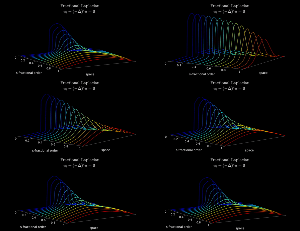
ssline = linspace(0.01,0.99,10);

iter = 0;
for s = ssline
    iter = iter + 1;
    A = -FEFractionalLaplacian(s,1,N);
    dynamics.A = A;
    [Ysolution] = solve(dynamics,U0);
    Data(iter).Y = Ysolution';
end
animation_FLD(ssline,Data,xline)

References
[1] U. Biccari and V. Hernández-Santamaría - Controllability of a one-dimensional fractional heat equation: theoretical and numerical aspects, IMA J. Math. Control. Inf., to appear