Moving control strategy for memory-type equations

Download Code

This tutorial shows how to implement the moving control strategy for the heat equation in the presence of a memory term.

The standard null controllability problem for the heat equation reads as follows

$\label{heatinterior} \begin{equation} \begin{cases} \begin{matrix} u_t = \Delta u + f(x,t) \chi_{\omega} \ & \ x \in \Omega & t \in [0,T] \\ u(x,t) = 0 & x \in \partial \Omega & t \in [0,T] \\ u(x,0) = u_0 & x \in \Omega \end{matrix} \end{cases}, \end{equation}$

where $\Omega$ is a bounded domain, $u_0\in L^2(\Omega)$ and the control $f$ acts on the subdomain $\omega\subset\Omega$. The objective is to steer the system from $u_0$ to zero in time $T$,

It is known that the null controllability of the heat equation holds in any positive time $T>0$ and for any open control region $\omega$. Nevertheless, the situation changes when in the model appears a memory term:

$\label{heatinterior_memory} \begin{equation} \begin{cases} \begin{matrix} \displaystyle u_t = \Delta u + f(x,t) \chi_{\omega} + \int_0^t u(x,\tau) d\tau \ & \ x \in \Omega & t \in [0,T] \\ u(x,t) = 0 & x \in \partial \Omega & t \in [0,T] \\ u(x,0) = u_0 & x \in \Omega \end{matrix} \end{cases} \end{equation}$

As a matter of fact, when the equation involes a memory term, it is impossible to achive null controllability in the classical sense, unless the control region coincides with the entire domain ($\omega=\Omega$).

This fact can be easily seen when applying a LQR control on both systems (\ref{heatinterior}) and (\ref{heatinterior_memory}). In the former case (without memory) the minimum of the LQR functional is an optimal control stabilizing the dynamics (Video 1), whereas when the memory enters into the model this minimum leaves the system far from the equilibrium (Vdeo 2).


Video 1: LQR in the heat equation (Equation \ref{heatinterior})	Video 2: LQR in the heat equation with memory (Equation \ref{heatinterior_memory})
We can see the time evolution of the two models with a control region, $\chi_{\omega}$, located in the position of the blue ellipsoid in the simulation. We observe that the LQR control is effective for the heat equation but not for the heat equation with memory.

To understand the reason behind the lack of null controllability for the memory-type equation (\ref{heatinterior_memory}), we can introduce the new variable

$z(x,t) = \int_0^t u(x,\tau) d\tau \Rightarrow z_t(x,t) = u(x,t)$

In this way, (\ref{heatinterior_memory}) is transformed into a coupled PDE/ODE system:

$\label{heatinterior_memory_z} \begin{equation} \begin{cases} \begin{matrix} u_t = \Delta u + f(x,t) \chi_{\omega} + z, & z_t = u & x \in \Omega & t \in [0,T] \\ u(x,t) = 0, & z(x,t) = 0 & x \in \partial \Omega & t \in [0,T] \\ u(x,0) = 0 & z(x,0) = 0 & x \in \Omega \end{matrix} \end{cases} \end{equation}$

In (\ref{heatinterior_memory_z}), the equation $z_t = u$ is an infinte-dimensional ODE which, since it has no diffusion term, introduces non-propagation phenomena in the system. The non propagating components corresponding to this ODE are unable to reach the control region $\omega$ and, therefore, cannot be controlled.

A natural remedy to this issue is to operate with a moving control strategy. If the ODE components of the system cannot reach the control region $\omega$, then is the control region who needs to reach these components. Hence, our control region would be function of the time variable, $\omega = \omega(t)$, and the corresponding model will be

$\label{heatinterior_memory_z_moving} \begin{equation} \begin{cases} \begin{matrix} u_t = \Delta u + f(x,t) \chi_{\omega(t)} + z, & z_t = u & x \in \Omega & t \in [0,T] \\ u(x,t) = 0, & z(x,t) = 0 & x \in \partial \Omega & t \in [0,T] \\ u(x,0) = 0 & z(x,0) = 0 & x \in \Omega \end{matrix} \end{cases} \end{equation}$

This moving control strategy has been proposed and succesfully applied in several contributions of our team [1,2,3,4].

Memory-type equations are one of the core topics of WP5 of the DyCon ERC project. An abridged presentation of this working package can be found at the following link.

Numerical implementation of the moving control strategy

We present here the numerical implementation of the moving control strategy for the memory-type heat equation (\ref{heatinterior_memory_z_moving}). All the simulations will be in $2D$.

STEP 1: construction of the control region

The first step is to construct the moving control region $\omega(t)$, which requires to design the function $\chi_{\omega(t)}$. To this end, we made the assumption that the size and orientation of $\omega(t)$ do not change during the time interval $[0,T]$. Hence, once fixed the size and shape of the control region, we will obtain a function depending only on a point $x\in \Omega$.

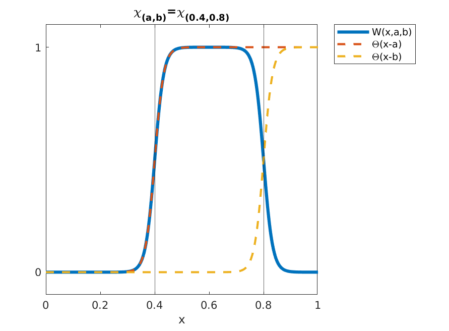
In this simulation, we create the control region as a square which moves in the domain $\Omega$. This square can be constructed with a function $W(x)$ defined as

$W(x,a,b) = H(x-a) + H(x-b) \\ \{ a,b,x \}\in \mathbb{R}, \quad a>b \\$

where $H(x)$ is the Heaviside function. Nevertheless, the function $W$ constructed in this way would be non-differentialbe at the points $x=a$ and $x=b$. This would represent a problem when implementing the gradient method to compute the control. To bypass this issue, in the definition of $W(x,a,b)$ we will use a smooth approximation of $H$ (See Figure 1).


Figure 1: Graphicla representation of $W(x,a,b)$

Moreover, the generalization of this function to dimension two is immediate

$W_{2D}(x,y,x_{min},x_{max},y_{min},y_{max}) = W(x,x_{min},x_{max})*W(x,y_{min},y_{max})$

In this way, given $(x_{min}, x_{max}, y_{min}, y_{max})$, we obtain the corresponding characteristic function which only depends on the position of a single point.

STEP 2: construction of the dynamics

Since $\chi_{\omega}$ can move and, moreover, we want to obtain the optimal trajectory for the control, we will incorporate in our system a moving particle whose position and velocity are denoted by $\textbf{d} = (d_x,d_y)$ and $\textbf{v} = (v_x,v_y)$, respectively (Video 3).


Video 3: Representación gráfica de $W_{2D}$

Besides, we will add a control $\textbf{g}(t) = (g_x(t),g_y(t))$ which will act as an exterior force moving the subset $\chi_{\omega}$.

In this way, our model takes the final form

$\label{heatinterior_memory_z_all} \begin{equation} \begin{cases} \begin{matrix} u_t = \Delta u + f(x,t) \chi_{\omega(\textbf{d})} + z, & z_t = u & x \in \Omega & t \in [0,T] \\ u(x,t) = 0, & z(x,t) = 0 & x \in \partial \Omega & t \in [0,T] \\ u(x,0) = 0, & z(x,0) = 0 & x \in \Omega \\ \dot{\textbf{d}} = \textbf{v} & \textbf{d}(0) = \textbf{d}_0 & t \in [0,T]\\ \dot{\textbf{v}} = \textbf{g}(t) & \textbf{v}(0) = \textbf{v}_0 & t \in [0,T]\\ \end{matrix} \end{cases} \end{equation}$

STEP 3: optimal control problem

Following a standard optimal control strategy, the control function for our memory-type equation will be computed throught the minimization problem

$\min_{f(x,t),g(t)} \|u(x,T)\|^2_{L^2(\Omega)} \\$ $\text{subject to: }\quad \begin{cases} \begin{matrix} u_t = \Delta u + f(x,t) \chi_{\omega(\textbf{d})} + z, & z_t = u & x \in \Omega & t \in [0,T] \\ u(x,t) = 0, & z(x,t) = 0 & x \in \partial \Omega & t \in [0,T] \\ u(x,0) = 0, & z(x,0) = 0 & x \in \Omega \\ \dot{\textbf{d}} = \textbf{v} & \textbf{d}(0) = \textbf{d}_0 & t \in [0,T]\\ \dot{\textbf{v}} = \textbf{g}(t) & \textbf{v}(0) = \textbf{v}_0 & t \in [0,T]\\ \end{matrix} \end{cases}$

Simulations

All the simulations in this tutorial have been performed using the DyCon Toolbox and CasADi. Since CasADi is incorporated into the DyCon toolbox, we can install it in the following way:

unzip('https://github.com/DeustoTech/DyCon-Computational-Platform/archive/master.zip')
addpath(genpath(fullfile(cd,'DyCon-toolbox-master'))
StartDyconPlatform

We shall now write the discrete version of equation (\ref{heatinterior_memory_z_all}):

$\label{heatinterior_memory_z_all_discr} \begin{equation} \frac{d}{dt} \begin{bmatrix}\begin{array}{c|c} \textbf{U} \\ \hline \textbf{Z} \\ \hline \textbf{D} \\ \hline \textbf{V} \\ \end{array} \end{bmatrix} = \begin{bmatrix}\begin{array}{c|c|c} \mathcal{A} & \textbf{1} & \textbf{0} & \textbf{0} \\ \hline \textbf{1} & \textbf{0} & \textbf{0} & \textbf{0} \\ \hline \textbf{0} & \textbf{0} & \textbf{0} & \textbf{1} \\ \hline \textbf{0} & \textbf{0} & \textbf{0} & \textbf{0} \\ \end{array} \end{bmatrix} %% \begin{bmatrix}\begin{array}{c|c} \textbf{U} \\ \hline \textbf{Z} \\ \hline \textbf{D} \\ \hline \textbf{V} \\ \end{array} \end{bmatrix} + %% \begin{bmatrix}\begin{array}{c|c} \textbf{B}(\textbf{D})*\textbf{F}(t) \\ \hline \textbf{0} \\ \hline \textbf{0} \\ \hline \textbf{G}(t) \\ \end{array} \end{bmatrix} \end{equation}$

Secondly, let us create the mesh variable

% Create the mesh variables
clear;
Ns = 7;
Nt = 15;
xline = linspace(-1,1,Ns);
yline = linspace(-1,1,Ns);
[xms,yms] = meshgrid(xline,yline);

and the matrix $A$ containing the $2D$ Laplacian and the ODE dynamics

A  = FDLaplacial2D(xline,yline);

Atotal = zeros(2*Ns^2+4,2*Ns^2+4);
%
Atotal( 1:Ns^2  , 1:Ns^2 ) = A;
%
Atotal( Ns^2+1 : 2*Ns^2   ,   1    :  Ns^2   )  =  eye(Ns^2);
Atotal(    1   :  Ns^2    , Ns^2+1 : 2*Ns^2  )  =  50*eye(Ns^2); % z = 50*y

RumbaMatrixDynamics = [0 0 1 0; ...
                       0 0 0 1; ...
                       0 0 0 0; ...
                       0 0 0 0 ];

Atotal(2*Ns^2+1:end,2*Ns^2+1:end) = RumbaMatrixDynamics;
Atotal = sparse(Atotal);

Finally, we create the function $B(\textbf{d}) = B(x_d,y_d)$ for the dynamics of the moving control

%%
% We create the B() function
xwidth = 0.3;
ywidth = 0.3;
B = @(xms,yms,xs,ys) WinWP05(xms,xs,xwidth).*WinWP05(yms,ys,ywidth);
Bmatrix =  @(xs,ys) [diag(reshape(B(xms,yms,xs,ys),1,Ns^2)) ;zeros(Ns^2)];

We now have everything we need to construct and solve the optimal control problem

opti = casadi.Opti();  % CasADi optimization structure

% ---- Input variables ---------
Ucas = opti.variable(2*Ns^2+4,Nt+1); % state trajectory
Fcas = opti.variable(Ns^2+2,Nt+1);   % control

% ---- Dynamic constraints --------
dUdt = @(y,f) Atotal*u+ [Bmatrix(u(end-3),u(end-2))*f(1:end-2) ; ...
                                         0                     ; ...
                                         0                     ; ...
                                     f(end-1)                  ; ...
                                     f(end)                    ]; 

% -----Euler backward method-------
for k=1:Nt % loop over control intervals
   y_next = Ucas(:,k) + (T/Nt)*dUdt(Ucas(:,k+1),dUdt(:,k+1)); 
   opti.subject_to(Ucas(:,k+1)==y_next); % close the gaps
end

% ---- State constraints --------
opti.subject_to(Ucas(:,1)==[Y0 ; 0.7 ; 0.7; -1.5 ; -1.5]);

% ---- Optimization objective  ----------
Cost = (Ucas(1:end-4,Nt+1))'*(Ucas(1:end-4,Nt+1));

opti.minimize(Cost); % minimizing L2 at the final time

% ---- initial guesses for solver ---
opti.set_initial(Ucas, Unum_free);
opti.set_initial(Fcas, 0);

% ---- solve NLP              ------
p_opts = struct('expand',false);
s_opts = struct('acceptable_tol',1e-4,'constr_viol_tol',1e-3,'compl_inf_tol',1e-3);
opti.solver('ipopt',p_opts,s_opts); % set numerical backend
tic
sol = opti.solve();   % actual solve
toc

The following video shows the results of our simulations, which allowed to compute an effective moving control steering the dynamics to rest at time $T$.


Video 3

Bibliography

[1] U. Biccari and S. Micu, Null-controllability properties of the wave equation with a second order memory term, J. Differential Equations, 267(2), 2019, 1376-1422.

[2] U. Biccari and M. Warma, Null-controllability properties of a fractional wave equation with a memory term, Evol. Eq. Control The., 9(2), 2020, 399-430.

[3] F. W. Chaves-Silva, X. Zhang and E. Zuazua, Controllability of evolution equations with memory, SIAM J. Control Optim., 55(4), 2017, 2437–2459.

[4] Q. Lü, X. Zhang and E. Zuazua, Null controllability for wave equations with memory, J. Math. Pures Appl., 108 (4), 2017, 500-531.

Simulation of Fractional Heat Equation

In this tutorial, we show the simulation of heat fractional equation

Author: Umberto Biccari - 01 February 2020

Optimal Control of the Fokker-Planck Equation with CasADi

In this tutorial, we present an optimal control problem related to the Fokker-Planck equation.

Author: Jorge Mallo - 19 December 2019

Numerical simulation of nonlinear Population Dynamics Structuring by age and Spatial diffusion

In this tutorial, we propose the Hum method to approximate numerically the control in a null controllability problem for a non linear population dynamics model structuring in age and spatial diffusion.

Author: Yacouba Simpore - 30 October 2019

Controllability of a Class of Infinite Dimensional Systems with Age Structure

In this tutorial, we investigate the linear infinite dimensional system obtained by implementing an age structure to a given linear dynamical system. We show that if the initial system is null controllable in a time small enough, then the age structured system is also null controllable in a time depending on the various involved parameters.

Author: Debayan Maity - 07 June 2019

Work Packages ≻ Models involving memory terms and hybrid PDE+ODE systems ≻