Download Code
In this tutorial we will present a simultaneous control problem in a linear system dependent on parameters. We will use the MATLAb DyCon Toolbox library.
Setup
In this tutorial we need DyCon Toolbox, to install it we will have to write the following in our MATLAB console:
unzip('https://github.com/DeustoTech/DyCon-Computational-Platform/archive/master.zip')
addpath(genpath(fullfile(cd,'DyCon-toolbox-master')))
StartDyConToolbox
You can see the code of this tutorial write the following line:
open T06ODET0002_Simultaneous
Problem definition
The simultaneous control problem is defined as:
subject to:
where:
Numerical Implementation
First we import the CasAdi library in order to create symbolic variables
import casadi.*
%% In this case $\nu_i$ are
M = 50;
nu = linspace(1,6,M);
Then we create the matrices of linear dynamics.
With these matrices we create the ode object
Nt = 500;T  = 0.8;
tspan = linspace(0,T,Nt);
%% create linear dynamic
iode = linearode(A,B,tspan);
%% set initial condition
Y0 = ones(2, 1);
iode.InitialCondition = repmat(Y0,M,1);
then we create the optimal control problem
% Get Symbolical variable
Ys  = iode.State.sym;
Us  = iode.Control.sym;
ts  = SX.sym('t'); %% <= Create a symbolical time
% Set Target
YT = zeros(2, 1);YT = repmat(YT,M,1);
%
PathCost  = casadi.Function('L'  ,{ts,Ys,Us},{ (1/2)*(Us'*Us)           });
FinalCost = casadi.Function('Psi',{Ys}      ,{  1e7*((Ys-YT).'*(Ys-YT)) });
% Create the optimal control
iocp = ocp(iode,PathCost,FinalCost);
Solve Optimal Control Problem with ipopt solver
U0 = ZerosControl(iode);
[Uopt ,Yopt] =  IpoptSolver(iocp,U0);
This is Ipopt version 3.12.3, running with linear solver mumps.
NOTE: Other linear solvers might be more efficient (see Ipopt documentation).

Number of nonzeros in equality constraint Jacobian...:   199700
Number of nonzeros in inequality constraint Jacobian.:        0
Number of nonzeros in Lagrangian Hessian.............:      600

Total number of variables............................:    50500
                     variables with only lower bounds:        0
                variables with lower and upper bounds:        0
                     variables with only upper bounds:        0
Total number of equality constraints.................:    50000
Total number of inequality constraints...............:        0
        inequality constraints with only lower bounds:        0
   inequality constraints with lower and upper bounds:        0
        inequality constraints with only upper bounds:        0

iter    objective    inf_pr   inf_du lg(mu)  ||d||  lg(rg) alpha_du alpha_pr  ls
   0  1.0000000e+09 1.12e-02 7.88e+00  -1.0 0.00e+00    -  0.00e+00 0.00e+00   0
   1  4.0934345e+06 1.26e-13 5.63e-09  -1.0 1.66e+02    -  1.00e+00 1.00e+00f  1

Number of Iterations....: 1

                                   (scaled)                 (unscaled)
Objective...............:   2.0467172272726700e+01    4.0934344545453396e+06
Dual infeasibility......:   5.6305735629536002e-09    1.1261147125907198e-03
Constraint violation....:   1.2612133559741778e-13    1.2612133559741778e-13
Complementarity.........:   0.0000000000000000e+00    0.0000000000000000e+00
Overall NLP error.......:   5.6305735629536002e-09    1.1261147125907198e-03


Number of objective function evaluations             = 2
Number of objective gradient evaluations             = 2
Number of equality constraint evaluations            = 2
Number of inequality constraint evaluations          = 0
Number of equality constraint Jacobian evaluations   = 2
Number of inequality constraint Jacobian evaluations = 0
Number of Lagrangian Hessian evaluations             = 1
Total CPU secs in IPOPT (w/o function evaluations)   =      1.391
Total CPU secs in NLP function evaluations           =      0.027

EXIT: Optimal Solution Found.
               t_proc [s]   t_wall [s]    n_eval
       nlp_f     0.000381      0.00038         2
       nlp_g       0.0042       0.0042         2
  nlp_grad_f      0.00167      0.00167         3
  nlp_hess_l      0.00331      0.00332         1
   nlp_jac_g        0.026        0.026         3
      solver         1.48         1.36         1
Elapsed time is 3.853462 seconds.
Compute Free solution
Yfree = solve(iode,U0*0);
Yfree = full(Yfree);
Visualization
fig = figure;
fig.Units = 'norm';fig.Position = [0.1 0.1 0.6 0.5];
%%
plotSimu(tspan,Yfree,Yopt,Uopt,M)
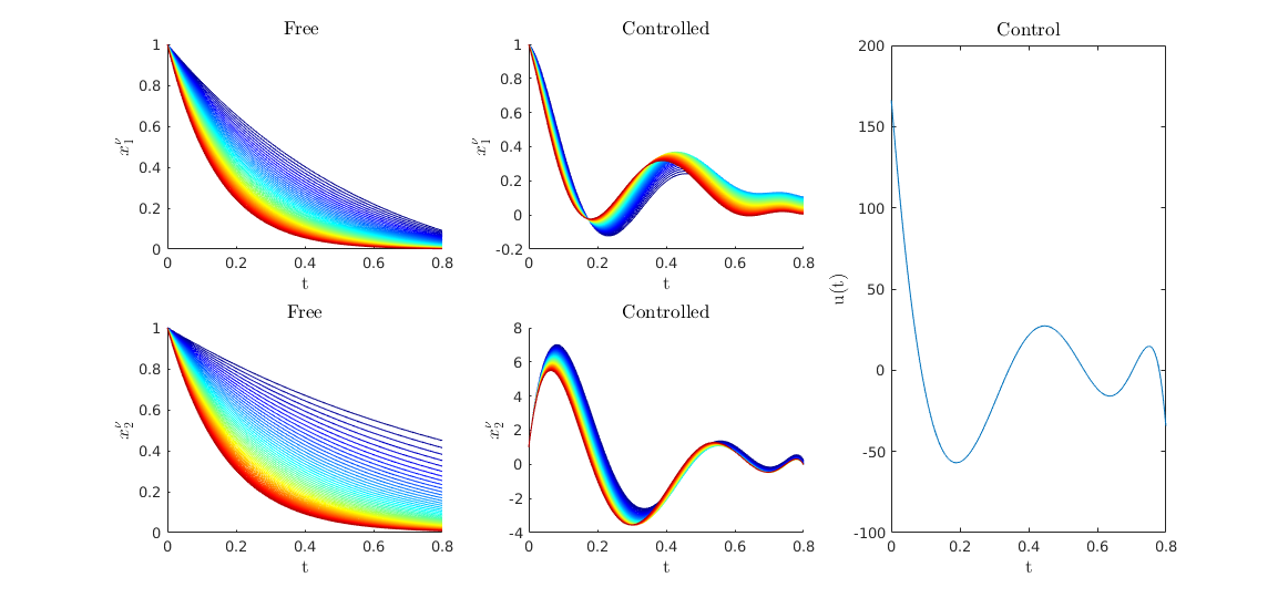
Figure 1. The different colors represent the dynamic system under different parameters. It can be seen how the same control is obtained acting for all the dynamic systems is capable of driving the systems to the target.