Synchronized Oscillators

Download Code

Consider the Kuramoto model for the synchronization of coupled oscillators

$$\begin{cases} \displaystyle \dot{\theta}_i(t) = \omega_i + \frac{Ku(t)}{N}\sum_{j=1}^N \sin \big(\theta_j(t)-\theta_i(t)\big),\quad i = 1,\ldots,N,\quad t>0 \\ \theta_i(0) = \theta_i^0. \end{cases}\quad (1)$$

Here $\theta_i(t)$, $i = 1,\ldots,N$, is the phase of the $i$-th oscillator, $\omega_i$ is its natural frequency and $K$ is the coupling strength. The frequencies $\omega_i$ are distributed with a given probability density $f(\omega)$, unimodal and symmetric around the mean frequency

$$\Omega = \frac 1N \sum_{i=1}^N \omega_i,$$

that is, $f(\Omega+\omega) = f(\Omega-\omega)$.

It is known that, if the coupling $K$ is sufficiently strong, the oscillators will synchronize asymptotically, i.e.

$$\lim_{t\to +\infty} |\dot{\theta}_i(t)-\dot{\theta}_j(t)| = 0, \quad \textrm{ for all }\; i,j = 1,\ldots,N,$$

We want to design a control capable to ensure synchronization in a final time horizon $T$, that is

$$|\dot{\theta}_i(T)-\dot{\theta}_j(T)| = 0, \quad \textrm{ for all } i,j = 1,\ldots,N. \quad\quad\quad(2)$$

To compute this optimal control allowing us to reach the synchronized configuration (3) we can adopt a classical approach based on the resolution of the following optimization problem

$$\begin{array}{l} \displaystyle\widehat{u} = \min_{u\in L^2(0,T;\mathbb{R})} J(u) \\[10pt] \displaystyle J(u) = \frac{1}{2} \sum_{i,j=1}^N \sin^2\big(\theta_j(T)-\theta_i(T)\big) + \frac \beta2 \|u\|^2_{L^2(0,T;\mathbb{R})}, \end{array}\quad (3)$$

subject to the dynamics (1).

For the resolution of (3), we use the standard GD method, which looks for the minimum $u$ as the limit $k\to +\infty$ of the following iterative process

$$u^{k+1} = u^k - \eta_k\nabla J(u^k). \quad (4)$$

This gradient technique is most often chosen because it is very easy to be implemented.

In order to fully define the iterative scheme (4), we need to compute the gradient $\nabla J(u)$. This can be done via the Pontryagin maximum principle.

To this end, let us first rewrite the dynamics (1) in a vectorial form as follows

$$\begin{cases} \dot{\Theta}(t) = \Omega + F\big(\Theta(t),u(t)\big), \quad t>0 \\ \Theta(0) = \Theta^0, \end{cases}$$

with $\Theta :=(\theta_1,\ldots,\theta_N)^\top$, $\Theta^0:=(\theta_1^0,\ldots,\theta_N^0)^\top$ and $\Omega :=(\omega_1,\ldots,\omega_N)^\top$, and where $F$ is the vector field given by

$$F = (F_1,\ldots,F_N), \quad F_i:= \frac{Ku(t)}{N}\sum_{j=1}^N\sin\big(\theta_j(t)-\theta_i(t)\big), \quad i=1,\ldots,N.$$

Using the notation just introduced, we obtain the following expression for the gradient of $J(u)$

$$\nabla J(u) = \beta u + (\mathcal D_uF)^\top p, \quad(5)$$

where $\mathcal D_uF$ indicates the Jacobian of the vector field $F$, computed with respect to the variable $u$.

In (5), we denoted with $p = (p_1,\ldots,p_N)$ the solution of the adjoint equation associated with (1), which is given by

$$\begin{cases} -\dot{p} = (\mathcal D_{\Theta}F)^\top p \\ p(T) = \nabla_{\Theta(T)}\phi(\Theta(T)), \end{cases}$$

where $\mathcal D_\Theta F$ stands again for the Jacobian of the vector field $F$, this time computed with respect to the variable $\Theta$.

Taking into account the expression of the vector field $F$, we can then see that the iterative scheme (4) becomes

$$u^{k+1} = u^k -\eta_k\left[\beta u^k + \frac KN\sum_{i=1}^N p_i\left(\sum_{j=1}^N \sin(\theta_j-\theta_i)\right)\right], \quad (6)$$

with

$$\begin{cases} \displaystyle-\dot{p}_i = -\frac{Kup_i}{N}\sum_{i\neq j=1}^N \cos\big(\theta_j-\theta_i\big) + \frac{Ku}{N}\sum_{i\neq j=1}^N p_j \cos\big(\theta_j-\theta_i\big),\quad i = 1,\ldots,N,\quad t>0 \\[20pt] \displaystyle p_i(T) = \frac 12\sum_{i\neq j=1}^N \sin\big(2\theta_i(T)-2\theta_j(T)\big). \end{cases}$$

We then see that, at each iteration $k$ the optimization scheme (6) requires to solve a $N$-dimensional non-linear dynamical system. This may rapidly become computationally very expensive, especially when the number $N$ of oscillators in our system is large.

In order to reduce this computational burden, we can combine the standard GD algorithm with the so-called Random Batch Method (RBM), which is a recently developed approach (see [2]) allowing for an efficient numerical simulation of high-dimensional collective behavior problems. This technique is based on the following simple idea: at each time step $t_m = m\cdot dt$ in the mesh we employ to solve the dynamics, we divide randomly the $N$ particles into $n$ small batches with size $2\leq P<N$, denoted by $C_q$, $q = 1,\ldots,n$, that is

$$\begin{array}{l} C_q = \{i_{q_1},\ldots,i_{q_P}\}\subset \{1,\ldots,N\}, & & for\; all\; q = 1,\ldots,n \\[8pt] C_q\cap C_r = \emptyset, & & for\; all\; q,r = 1,\ldots,n \\[8pt] \bigcup_{q = 1}^n C_q = \{1,\ldots,N\}. \end{array}$$

Once this partition of ${1,\ldots,N}$ has been performed, we solve the dynamics by interacting only particles within the same batch. In this way, we are now dealing with systems of lower dimension and the computational cost of the GD algorithm is reduced.

Numerical simulations

We can check the effectiveness of the proposed approach through some numerical simulations for the computation of the optimal control $\widehat{u}$.

Firstly, we can show that the optimization problem (3) indeed allows to compute an effective control function which is capable to steer the Kuramoto model (1) to a synchronized configuration.

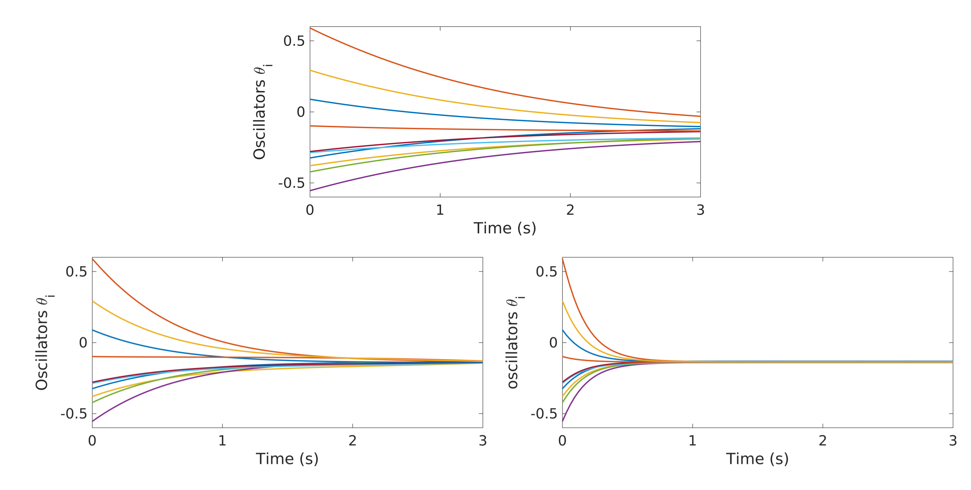
In Figure 1-top, we show the evolution of the uncontrolled dynamics, which corresponds to taking $u\equiv 1$ in (1). As we can see, the oscillators are evolving towards a synchronized configuration, but synchronization is not reached in the short time horizon we are providing. In Figure 1-bottom, we show the evolution of the same dynamics, this time under the action of the control function $u$ computed through the minimization of $J(u)$. The subplot on the left corresponds to the simulations done with the GD approach, while the one on the right is done employing GD-RBM. We can clearly see how, in both cases, the oscillators are all synchronized at the final time $T=3s$. This means that both algorithms managed to compute an effective control.

Figure 1. Top - evolution of the free dynamics of the Kuramoto model (1) with $N=10$ oscillators. Bottom - evolution of the controlled dynamics of the Kuramoto model (1) with $N=10$ oscillators. The control function $\widehat{u}$ is obtained with the GD (left) and the GD-RBM (right) approach.

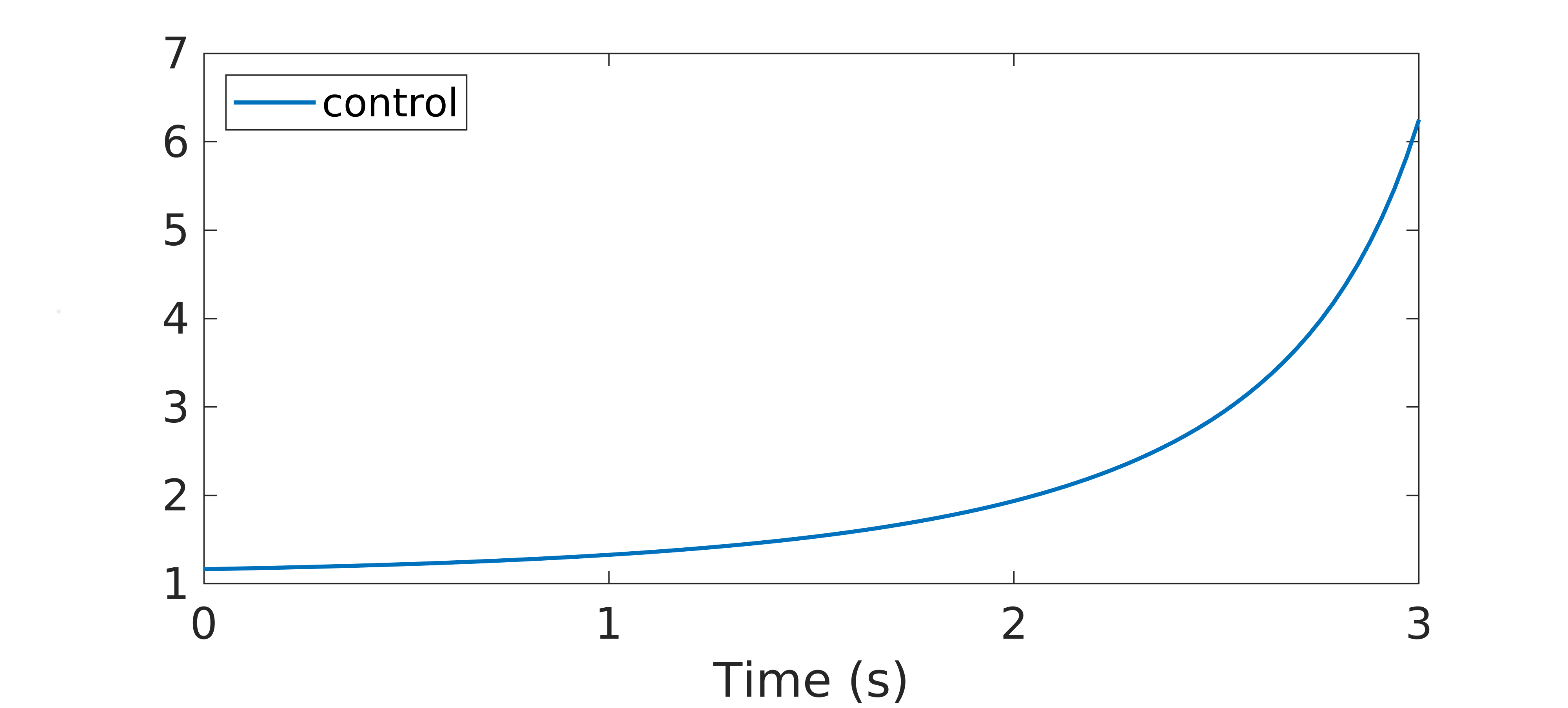
In Figure 2, we display the behavior of the control function $\widehat{u}$ computed via the GD-RBM algorithm. We can see how, at the beginning of the time interval we are considering, this control is close to one and it is increasing with a small slope. On the other hand, this growth becomes more pronounced as we get closer to the final time $T=3s$.

Figure 2. control function $\widehat{u}$ obtained through the GD-RBM algorithm applied to the Kuramoto model (1) with $N=10$ oscillators.

Notice that, in (1), $\widehat{u}$ enters as a multiplicative control which modifies the strength of the coupling $K$. Hence, according to the profile displayed in Figure 2, the control function $\widehat{u}$ we computed is initially letting the system evolving following its natural dynamics. Then, as the time evolves towards the horizon $T=3s$, $\widehat{u}$ enhances the coupling strength $K$ in order to reach the desired synchronized configuration (2).

We can now compare the performances of the GD and GD-RBM algorithms for the computation of the optimal control $\widehat{u}$. To this end, we can run simulations for increasing values of $N$, namely $N=10,50,100,250,1000$.

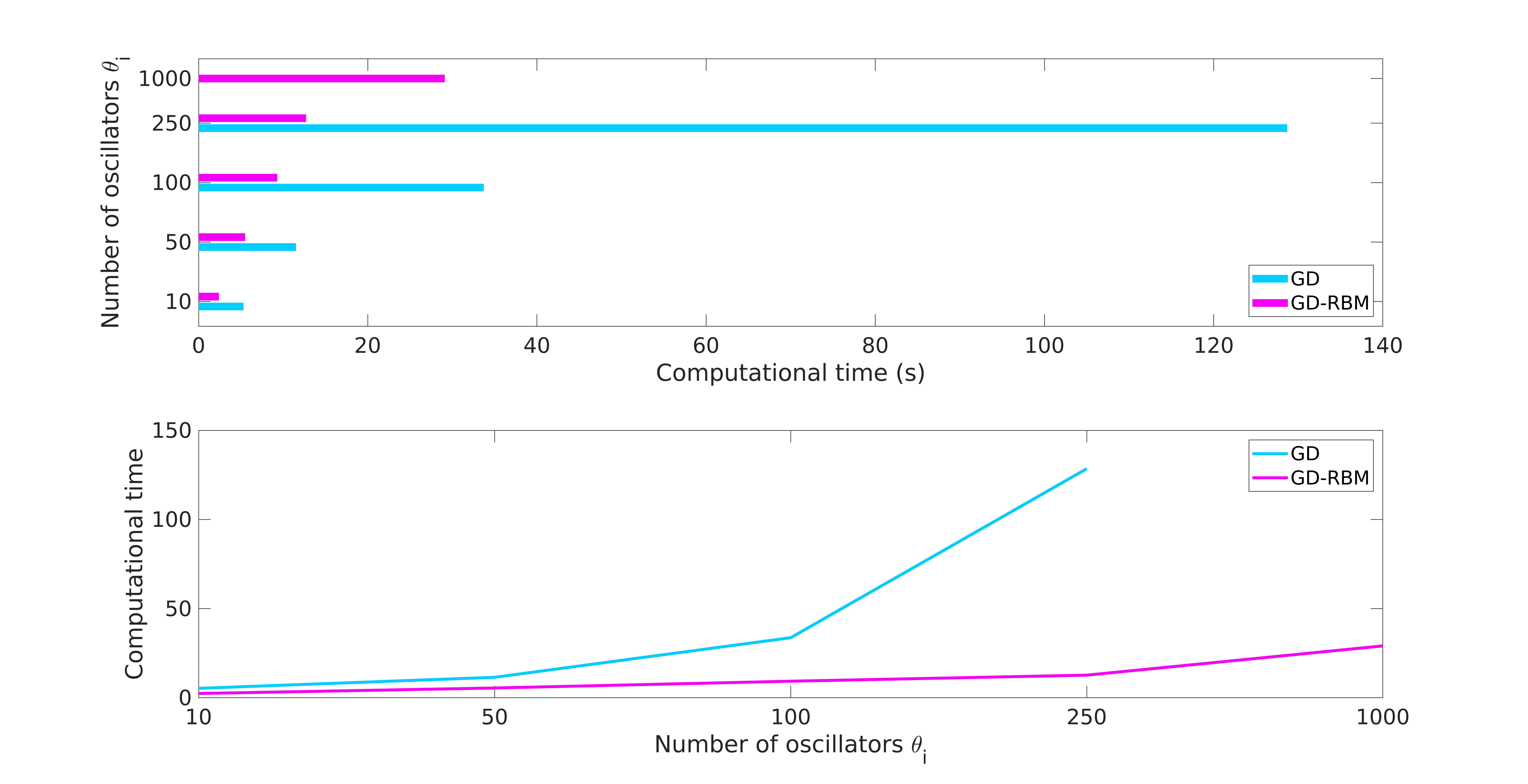
Figure Figure 3 shows the computational times required by the two methodologies to solve the optimization problem (3).

Figure 3. computational times required by the GD and GD-RBM algorithm to compute the optimal control $\widehat{u}$ with increasing values of $N$.

Our simulations show how, for low values of $N$, the two approaches show similar behaviors. Nevertheless, when increasing the number of oscillators in our system, the advantages of the GD-RBM methodology with respect to GD become evident. In particular, the growth of the computational time for GD-RBM is significantly less pronounced than for GD. As a matter of fact, Figure 3 is not considering the case of $N=1000$ oscillators with GD, since the behavior with smaller values of $N$ already suggested that this experiment would be computationally too expensive.

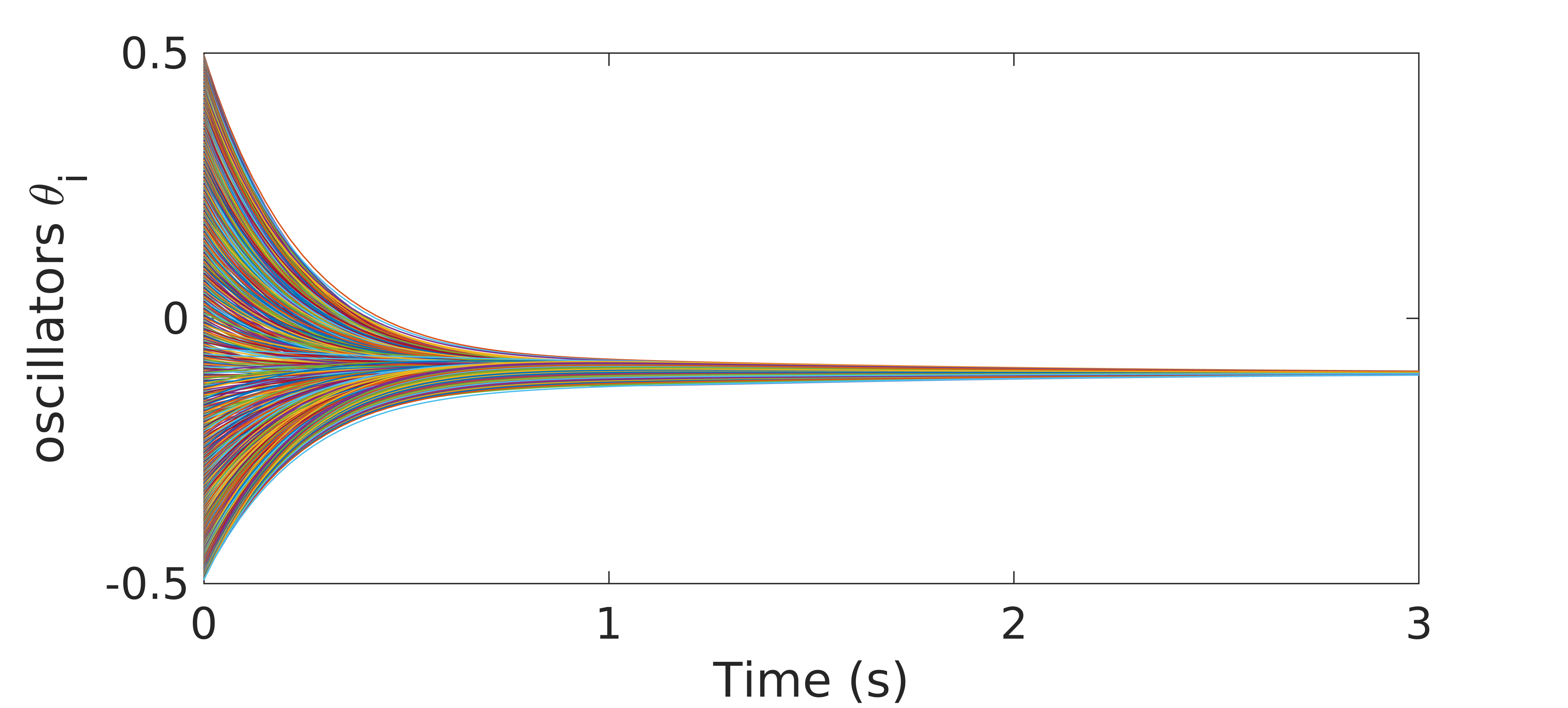
On the other hand, even with $N=1000$ oscillators in the system, the GD-RBM approach turns out to be able to compute an effective control for the Kuramoto model (1) in about $29$ seconds (see Figure 4).

Figure 4. evolution of the controlled dynamics of the Kuramoto model (1) with $N=1000$ oscillators. The control has been computed with the GD-RBM algorithm.

More details on the contents of this post can be found in [1].

Bibliography

[1] U. Biccari and E. Zuazua, A stochastic approach to the synchronization of coupled oscillators, to appear in Front. Energy Res.

[2] S. Jin, L. Li and J.-G. Liu, Random Batch Methods (RBM) for nteracting particle systems, J. Comput. Phys. 400 (2020), 108877.

---