DyCon Toolbox

MATLAB library for non-linear optimal control problems

The DyCon Toolbox is a MATLAB library for analyzing both linear and non-linear optimal control problems. It uses CasADi-based automatic differentiation to compute all derivatives necessary for the optimization process.

The DyCon Toolbox has a high-level syntax, which allows for an easy definition of the user’s control problem, and thus to its quick implementation. Moreover, the user may freely and easily tune the optimization algorithms in view of speeding-up the computation process.

The DyCon Toolbox provides two different approaches for tackling a control problem:

Direct method approach, which consists in discretizing both state and control. This reduces the original control problem to a nonlinear optimization problem (nonlinear programming). In this case, DyCon Toolbox provides a solution to the problem through optimization in IPOPT.
Indirect method approach, which consists in numerically solving the adjoint problem backwards in time, and computing the functional derivative of the problem. Gradient descent-based methods can then be used to obtain the optimal control.

Although direct methods are more common in the control community, when the problem is high dimensional, indirect methods are more efficient. The DyCon Toolbox unifies the definition of control problems so that they can be solved with the adequate method.

FEATURES

Sparse symbolic variables and automatic differentiation via CasADi
Direct method using Ipopt Solver
Indirect methods implemented (Pontryagin’s maximum principle)
Compatible with MATLAB PDE Toolbox
Easy to implement a new optimal control problems
Many numerical schemes already implemented (Runge Kutta methods)

A simple example

The simultaneous optimal control problem is defined as:

$\min _{u \in L^2(0,T)} \mathcal{J}\left( u\right) = \min _{u \in L^2(0,T)} \frac{1}{2} \sum_{\nu \in \mathcal{K}} || x\left( T, \nu \right) - x_T ||_{\mathbb{R}^ N}^2 + \frac{\beta}{2} \int_0^T u^2 \mathrm{d}t \quad \beta \in \mathbb{R}^+$

subject to:

$\left\{ \begin{array}{ll} x^\prime \left( t \right) = A \left( \nu \right) x \left( t \right) + B \left( \nu \right) u \left( t \right), \quad 0 < t <T, \\ x\left( 0 \right) = x^0. \end{array} \right.$

where:

$\mathcal{K}= \left\{ \nu_i \in \mathbb{R}, \enspace 1\leq i \leq K \right\}$

Numerical Implementation

We first import the CasAdi library in order to create symbolic variables

import casadi.*
M = 50; nu = linspace(1,6,M);

Then we create the matrices of linear dynamics.

$A_\nu = \begin{bmatrix} -\nu & 1 \\ 0 & -\nu \end{bmatrix} \ \ \ B_\nu = \begin{bmatrix} 0 \\ 1 \end{bmatrix}$

[A,B] = GenMatSim(nu);

With these matrices we create the ode object

% define the time span
Nt = 500;T  = 0.8;
tspan = linspace(0,T,Nt);
% create linear dynamic object
iode = linearode(A,B,tspan);
% set initial condition
Y0 = ones(2, 1);
iode.InitialCondition = repmat(Y0,M,1);

then we create the optimal control problem

% Get Symbolical variable
Ys  = iode.State.sym;
Us  = iode.Control.sym;
ts  = SX.sym('t'); %% <= Create a symbolical time
% Set Target
YT = zeros(2*M, 1);
%
PathCost  =  (1/2)*(Us'*Us)          ;
FinalCost =  1e7*((Ys-YT).'*(Ys-YT)) ;
% Create the optimal control
iocp = ocp(iode,PathCost,FinalCost);

We solve the Optimal Control Problem with an Ipopt solver

U0 = ZerosControl(iode);    % <= Control initial guess
[Uopt ,Yopt] =  IpoptSolver(iocp,U0);

This is Ipopt version 3.12.3, running with linear solver mumps.
NOTE: Other linear solvers might be more efficient (see Ipopt documentation).

Number of nonzeros in equality constraint Jacobian...:   199700
Number of nonzeros in inequality constraint Jacobian.:        0
Number of nonzeros in Lagrangian Hessian.............:      600

Total number of variables............................:    50500
                     variables with only lower bounds:        0
                variables with lower and upper bounds:        0
                     variables with only upper bounds:        0


iter    objective    inf_pr   inf_du lg(mu)  ||d||  lg(rg) alpha_du alpha_pr  ls
   0  1.0000000e+09 1.12e-02 7.88e+00  -1.0 0.00e+00    -  0.00e+00 0.00e+00   0
   1  4.0934345e+06 1.26e-13 5.63e-09  -1.0 1.66e+02    -  1.00e+00 1.00e+00f  1

Number of Iterations....: 1

...

EXIT: Optimal Solution Found.
               t_proc [s]   t_wall [s]    n_eval
       nlp_f     0.000381      0.00038         2
       nlp_g       0.0042       0.0042         2
  nlp_grad_f      0.00167      0.00167         3
  nlp_hess_l      0.00331      0.00332         1
   nlp_jac_g        0.026        0.026         3
      solver         1.48         1.36         1
Elapsed time is 3.853462 seconds.

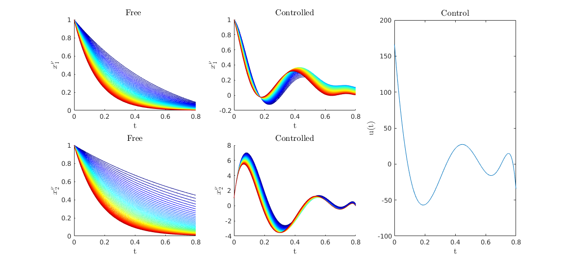
We can compute the free solution

Yfree = solve(iode,U0*0);
Yfree = full(Yfree);

Visualization

fig = figure();
%%
plotSimu(tspan,Yfree,full(Yopt),Uopt,M)

Figure 1. The different colors represent the dynamic system under different parameters. It can be seen how the same control is obtained acting for all the dynamic systems is capable of driving the systems to the target.