Download Code
In this tutorial, we present an optimal control problem related to the Fokker-Planck equation.
Description of the problem
The Fokker Planck Equation
Let $\Omega$ be an open, bounded, regular subset of $\mathbb{R}^{n}$. Let $T>0$ and denote by $u\in L^2(0,T;H^{1}(\Omega))^n$ a time-dependent vector field in $\Omega$. Consider a particle in $\Omega$ that moves with velocity $u(x,t)$ at each point $x\in\Omega$ in time $t\in(0,T)$. Suppose furthermore that the particle is subject to additive Brownian noise.
Let $p_0(x)$ be the probability density of the position of the particle at time $t=0$. Then, at every time $t>0$, the probability density $p(x,t)$ of the particle satisfies the Fokker-Planck equation [1]:
Where $\mathrm{n}$ is the outward unit normal vector field on $\partial\Omega$.
Fix a positive real number $a>0$ and introduce the family of admissible controls:
For every non-negative initial data $p_0\in H^{1}(\Omega)$ and every admissible control $u\in\mathcal{U}_{\mathrm{ad}}$, there is a unique solution $p\in\mathcal{C}([0,T];L^{2}(\Omega))\cap L^{2}(0,T;H^{1}(\Omega))$ to the previous problem such that $p(x,t)\geq 0$ for every $t\geq 0$ and almost every $x\in\Omega$ [2].
If, besides, $\int_{\Omega}p_{0}(x)dx=1$, then integrating by parts it’s easy to check that $\int_{\Omega}p(x,t)dx=1$ for every $t\geq 0$, so $p(.,t)$ is indeed a probability density on $\Omega$ for every $t\geq 0$.
Optimal Control
Fix a smooth reference trajectory $z:[0,T]\rightarrow\Omega$. Our objective is to find an admissible control $u\in\mathcal{U}_{\mathrm{ad}}$ that minimizes the following functional:
subject to:
where $\alpha,\beta$ and $\gamma$ are non-negative real
numbers. In [2] it is proven that there always exists a $u^{*}\in\mathcal{U}_{\mathrm{ad}}$ minimizing the previous functional among the family of admissible controls.
Numerical Simulation
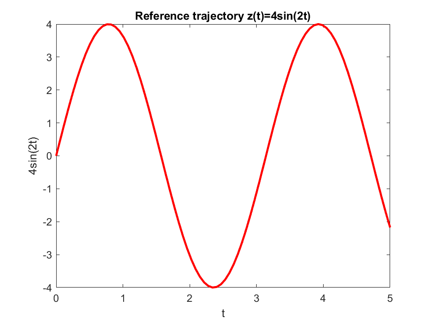
In the numerical example that we will present in this post, we will work over the one-dimensional domain $\Omega = (-6,6)$ with time horizon $T = 5$, and the oscillating reference trajectory $z(t) = 4\sin(2t)$. We also fix $\alpha=\beta=\gamma=1$, so that our objective will be to minimize the functional:
subject to
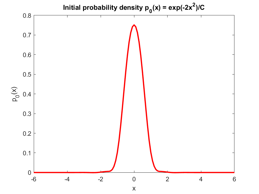
We consider the initial probability density function
where $C>0$ is chosen so that $\int_{-6}^{6}p_0(x)dx=1$.
We start by defining the mesh sizes and parameters. We discretize the spatial domain with $20$ points and the temporal domain with $80$ points.
%% mesh sizes and parameters

% spatial mesh
X_max = 6; % length of space domain
Nx = 20; % number of mesh points
x_line = linspace(-X_max,X_max,Nx); % discretization of the space domain
dx = x_line(2) - x_line(1); % space increment

% temporal mesh
T = 5; % time horizon
Nt = 80; % number of mesh points
t_line = linspace(0,T,Nt); % discretization of the time domain
dt = t_line(2) - t_line(1); % time increment

% parameters
k = dt/(dx^2);
b = dt/(2*dx);
We define the reference trajectory $z(t)=4\sin(2t)$:
%% reference trajectory

ref = 4*sin(2*t_line);
We define the initial probability density $p_0(x) = \frac{1}{C}\exp(-2x^2)$. We compute $C$ using $C = \int_{-6}^{6}\exp(-2x^2)dx = \sqrt{\frac{\pi}{2}}\mathrm{erf}(6\sqrt{2})$, where $\mathrm{erf}$ is the error function.
%% initial density

y0 = exp(-2*x_line.^2);

C = sqrt(pi/2)*erf(sqrt(2)*X_max); % normalizing constant
y0 = (1/C) * y0'; % normalized initial density
The uncontrolled evolution of this probability density is given by the following heat equation with Neumann boundary conditions:
We discretize and solve this equation:
%% uncontrolled solution

Yf = zeros(Nx,Nt);
Yf(:,1) = y0;

for n = 1 : Nt-1
    for j = 2 : Nx-1
        % euler step
        Yf(j,n+1) = Yf(j,n) +  k * (Yf(j+1,n) - 2*Yf(j,n) + Yf(j-1,n));
    end
    % zero flux boundary conditions
    Yf(Nx,n+1) = Yf(Nx-1,n+1);
    Yf(1,n+1) = Yf(2,n+1);
end
We display the uncontrolled solution:
The solution $p(x,t)$ of the Heat equation (2) is the probability density associated to a one-dimensional Brownian motion on the real line. This is a particular case of a more general phenomenon: there is a correspondence between certain second order parabolic equations and solutions of stochastic ordinary differential equations [3]. Using the computed value of $p(x,t)$, we can simulate sample paths of a Brownian motion on the real line: the following animation displays the evolution of $100$ Brownian particles without control:
We now set up the optimal control problem in CasADi:
%% optimal control problem

opti = casadi.Opti();
Y = opti.variable(Nx,Nt); % state variable
U = opti.variable(Nx,Nt); % control variable
We specify the system dynamics, discretizing the Fokker-Planck equation using central differences for the spatial derivatives and a forward Euler scheme for the time derivative:
%% system dynamics

for n = 1 : Nt-1
    for j = 2 : Nx-1
        term1 = k*(Y(j+1,n)-2*Y(j,n)+Y(j-1,n));
        term2 = b*Y(j,n)*(U(j+1,n)-U(j-1,n));
        term3 = b*U(j,n)*(Y(j+1,n)-Y(j-1,n));
        opti.subject_to(Y(j,n+1) == Y(j,n) + term1 - term2 - term3);
    end
end
We now set the initial condition and zero flux boundary conditions as constraints:
%% initial conditions and zero flux boundary conditions

% initial condition
opti.subject_to(Y(:,1) == y0);

% zero flux boundary conditions
for n = 2 : Nt
    opti.subject_to(Y(Nx,n) == Y(Nx-1,n)/(1-dx*U(Nx,n)));
    opti.subject_to(Y(1,n) == Y(2,n)/(1+dx*U(1,n)));
end
We set the constraints on the control, taking $a = 2$:
%% admissible control constraints

opti.subject_to(-2<=U(:)<=2);
We declare the cost functional:
%% cost functional

cost = 0;

% running cost
for n = 1 : Nt
    for i = 1 : Nx
        cost = cost + (x_line(i)-ref(n))^2*Y(i,n);
    end
end

% terminal cost
for i = 1 : Nx
    cost = cost + (x_line(i)-ref(n))^2*Y(i,Nt);
end

% control cost
for n = 1 : Nt % control cost
    for i = 1 : Nx
        cost = cost + Y(i,n)*U(i,n)^2;
    end
end
We solve the optimization problem using the IPOPT software:
%% solution of the optimization problem

% set optimization objective
opti.minimize(cost);

% solution of the optimization problem
p_opts = struct('expand',true);
s_opts = struct('max_iter',1000);
opti.solver('ipopt',p_opts,s_opts);

tic
sol = opti.solve();
toc
Obtaining the following display:
This is Ipopt version 3.12.3, running with linear solver mumps.
NOTE: Other linear solvers might be more efficient (see Ipopt documentation).

Number of nonzeros in equality constraint Jacobian...:    10448
Number of nonzeros in inequality constraint Jacobian.:     1600
Number of nonzeros in Lagrangian Hessian.............:     6204

Total number of variables............................:     3200
                     variables with only lower bounds:        0
                variables with lower and upper bounds:        0
                     variables with only upper bounds:        0
Total number of equality constraints.................:     1600
Total number of inequality constraints...............:     1600
        inequality constraints with only lower bounds:        0
   inequality constraints with lower and upper bounds:     1600
        inequality constraints with only upper bounds:        0

Number of Iterations....: 39

                                   (scaled)                 (unscaled)
Objective...............:  7.2472498957747769e+002   9.6893349411152292e+002
Dual infeasibility......:  1.0060574595627259e-010   1.3450657609300798e-010
Constraint violation....:  1.1102230246251565e-016   1.1102230246251565e-016
Complementarity.........:  2.5059036929760477e-009   3.3503108849024674e-009
Overall NLP error.......:  2.5059036929760477e-009   3.3503108849024674e-009


Number of objective function evaluations             = 40
Number of objective gradient evaluations             = 40
Number of equality constraint evaluations            = 40
Number of inequality constraint evaluations          = 40
Number of equality constraint Jacobian evaluations   = 40
Number of inequality constraint Jacobian evaluations = 40
Number of Lagrangian Hessian evaluations             = 39
Total CPU secs in IPOPT (w/o function evaluations)   =      1.062
Total CPU secs in NLP function evaluations           =      0.047

EXIT: Optimal Solution Found.
      solver  :   t_proc      (avg)   t_wall      (avg)    n_eval
       nlp_f  |   3.00ms ( 75.00us)   3.00ms ( 75.00us)        40
       nlp_g  |  14.00ms (350.00us)  13.99ms (349.85us)        40
  nlp_grad_f  |   5.00ms (121.95us)   5.00ms (121.90us)        41
  nlp_hess_l  |  10.00ms (256.41us)  10.01ms (256.74us)        39
   nlp_jac_g  |  15.00ms (365.85us)  15.98ms (389.78us)        41
       total  |   1.11 s (  1.11 s)   1.11 s (  1.11 s)         1
Elapsed time is 1.561797 seconds.
The following pictures display the temporal evolution of the controlled solution. The solution follows an oscillatory pattern similar to the one given by the reference trajectory:
Again, by the correspondence between second order parabolic equations and solutions to stochastic ordinary differential equations, the solution $p(x,t)$ to equation (2) is the probability density of a brownian particle on the real line that is subject to the velocity field $u(x,t)$. We use the values of $p(x,t)$ that we have just computed to simulate sample paths of this controlled brownian motion: the following animation displays the evolution of $100$ Brownian particles subject to the control $u(x,t)$:
References
[1] Hannes Risken, Till Frank. The Fokker-Planck Equation: Methods of Solution and Applications, Second Edition. Springer-Verlag Berlin Heidelberg, 1996
[2] Roy, S., Annunziato, M., Borzì, A., and Klingenberg, C. (2018). A Fokker–Planck approach to control collective motion. Computational Optimization and Applications, 69(2), 423-459.
[3] Stroock, Daniel W., Varadhan, S.R.S. Multidimensional Diffusion Processes. Springer-Verlag Berlin Heidelberg, Reprint of the 1997 Edition (Grundlehren der mathematischen Wissenschaften, Vol. 233).