Download Code
Infinite dimensional dynamical systems coupling age structuring with diffusion appear naturally in
population dynamics, medicine or epidemiology. A by now classical example is the Lotka-Mckendrick system with spatial diffusion. The
aim of this blog is to study contaollability properties of such age structured models in an unified manner.
Let $A : \mathcal{D}(A) \to X$ be the generator of a $C^0$ semigroup $\mathbb{S}$ on the Hilbert space $X$ and let $U$ be
another Hilbert space. Both $X$ and $U$ will be identified with their duals. Let $B$ be a (possibly unbounded) linear operator
from $U$ to $X$, which is supposed to be an admissible control operator for $\mathbb{S}$.
In the examples we have in mind, the above spaces and operators describe the dynamics of a system without age structure.
In particular, $X$ is the state space and $U$ is the control space.
The corresponding age structured system is obtained by first extending these spaces to
\begin{equation} \label{input-space}
\mathcal{X} = L^{2}(0,a_{\dagger}; X), \quad \mathcal{U} = L^{2}(0,a_\dagger;U).
\end{equation}
where $a_\dagger>0$ denotes the maximal age individuals can attain. Let $p(t) \in \chi$ be the distribution density of the
individuals with respect to age $a\geqslant 0$ and at some time $t \geqslant 0.$ Then the abstract version of the Lotka-McKendrick
system to be considered in this paper writes:
\begin{equation} \label{eq:main}
\begin{cases}
\displaystyle \frac{\partial p}{\partial t} + \frac{\partial p}{\partial a} - A p + \mu(a) p = \mathcal{\chi}_{(a_{1},a_{2})} B u, & t \geqslant 0, a \in (0,a_\dagger), \\
\displaystyle p(t,0) = \displaystyle \int_{0}^{a_\dagger} \beta(s) p(t,s) \; {\rm d}s, & t \geqslant 0, \\
\displaystyle p(0,a) = p_{0},
\end{cases}
\end{equation}
where $\mathcal{\chi}$ is the characteristic function of the interval $(a_{1}, a_{2})$ with
$0 \leqslant a_{1} < a_{2} \leqslant a_\dagger$ and $p_{0}$ is the initial population density.
In the above system, the positive function $\mu:[0,a_\dagger] \to \mathbb{R}_{+}$ denotes the
natural mortality rate of individuals of age $a.$ We denote by $\beta: [0,a_\dagger] \to \mathbb{R}_{+}$
the positive function describing the fertility rate at age $a.$ We assume that the fertility rate $\beta$ a
nd the mortality rate $\mu$ satisfy the conditions
- (H1) $\beta \in L^\infty[0, a_\dagger], \; \beta \geqslant 0$ for almost every $a \in [0,a_\dagger].$
- (H2) $\mu \in L^1_{loc}[0, a_\dagger], \; \mu \geqslant 0$ for almost every $a \in [0,a_\dagger].$
- (H3) $\displaystyle \int_0^{a_\dagger} \mu(a) \ {\rm d} a = \infty.$
Before we state our result, let us introduce the notion of null controllability of the pair $(A,B).$
We say that a pair $(A,B)$ is null-controllable in time $\tau,$ if for every $z_{0} \in X$ there exists a control $u \in L^{2}(0,\tau,U)$ such that, the solution of the system
\begin{equation*}
\dot z(t) = A z(t) + Bu(t) \quad t \in [0,\tau], \qquad z(0) = z_{0},
\end{equation*}
satisfies $z(\tau) = 0.$
We prove the following result
Assume that $\beta$ and $\mu$ satisfy the conditions (H1)-(H3) above. Moreover,
suppose that the fertility rate $\beta$ is such that
\begin{equation} \label{eq:beta}
\beta(a)= 0 \mbox{ for all } a \in (0,a_{b}),
\end{equation}
for some $a_b\in (0,a_\dagger)$ and that $a_1 < a_b$.
Let us assume that the pair $(A,B)$ is null controllable in arbitrary time.
Then for every $\tau > a_{1} + a_{\dagger}-a_{2}$ and for every $p_{0} \in \chi$ there exists a control $v \in L^{2}(0,\tau;\mathcal{U})$ such that the solution $p$ of \eqref{eq:main} satisfies
\begin{equation}
p(\tau,a) = 0 \mbox{ for all } a \in (0,a_\dagger).
\end{equation}
It is well known that null controllability is equivalent to final state observability of the adjoint system
(see for instance [4, Section 11.2]). The adjoint of the above system reads as
\begin{equation} \label{eq:adj}
\begin{cases}
\displaystyle \frac{\partial q}{\partial t} - \frac{\partial p}{\partial a} - A^* p + \mu(a) p - \beta(a) q(t,0) = 0, & t \geqslant 0, a \in (0,a_\dagger), \\
\displaystyle q(t,a_\dagger) = 0, & t \geqslant 0, \\
\displaystyle q(0,a) = q_{0},
\end{cases}
\end{equation}
where $A^*$ is the adjoint of $A.$ In order to prove Theorem 1, it is enough to prove the following
Let us assume the hypothesis of Theorem 1. Then for every $\tau > a_1 + a_\dagger - a_2$ there exists $k_\tau > 0$ such that
the solution $q$ of \eqref{eq:adj} satishfies
\begin{equation} \label{eq:est-adj}
\int_0^{a_\dagger} \|q(\tau, a)\|^2_X \ da \leqslant k_\tau^2 \int_0^\tau \int_{a_1}^{a_2} \left\|B^*q(t,a) \right\|^2_U \ da dt, \qquad \qquad (q_0 \in \mathcal{X}).
\end{equation}
Let us give an idea of the proof. We combine characteristics method with final state observability of the pair $(A^*, B^*).$ For siplicity
in the presentation, let us assume that $\mu = 0,$ $a_1 = 0,$ $a_2 < a_b$ and $\tau = 2a_\dagger.$
The detail proof of Theorem 1, in a slightly more general case, can be found in [3]. Integrating along the characteristic lines,
it is not very difficult to see that
\begin{equation*}
q(t,a) = \int_{t + a - a_\dagger}^{t} e^{(t-s)A^*} \beta(a+ \tau - s) q(s, 0) \ ds, \qquad t > a_\dagger.
\end{equation*}
Therefore,
\begin{equation} \label{est0}
\int_0^{a_\dagger} \|q(\tau, a)\|^2_X \ da \leqslant C \int_{a_\dagger}^\tau \left\|q(t,0) \right\|^2_X \ dt.
\end{equation}
Thus to prove \eqref{eq:est-adj}, we need to estimate the right hand side of the above estimate. We now make use of the condition
\eqref{eq:beta}. Note that, due to this condition, $q$ satisfies
\begin{equation} \label{eq:adj-2}
\displaystyle \frac{\partial q}{\partial t} - \frac{\partial q}{\partial a} - A^* p + \mu(a) p = 0, \quad t \geqslant 0, a \in (0,a_2).
\end{equation}
For a.e. $t \in (a_\dagger, \tau),$ we define $w(s) = q(s, t- s),$ $s \in (t - a_2, t).$ Then $w$ solves
\begin{equation*}
\displaystyle \frac{\partial w}{\partial s} - A^* w = 0, \quad s \in (t - a_2, t).
\end{equation*}
Since the pair $(A, B)$ is null controllable in any time, or equivalently the pair $(A^*, B^*)$ is final-state observable in any
time, there exists a constant
$C > 0,$ depending only on $a_2, A$ and $B$ such that
\begin{equation*}
\left\| w(t) \right\|_{X}^2 \leqslant C \int_{t-a_2}^t \left\| B^* w(s) \right\|^2_U \ ds.
\end{equation*}
Coming back to $q$ and integrating over $[a_\dagger, \tau]$ with respect to $t,$ we have that
\begin{equation}
\int_{a_\dagger}^\tau \|q(t,0)\|^2_X \ dt \leqslant \int_{0}^\tau \int_{0}^{a_2} \left\|B^* q(t,a)\right\|^2 \ da dt.
\end{equation}
Combining the above estimate together with \eqref{est0}, we get \eqref{eq:est-adj}. In the two figures below, we ilustrate the
estimate of $q(t,0)$ and the final-state observability of $q$ in the general case.
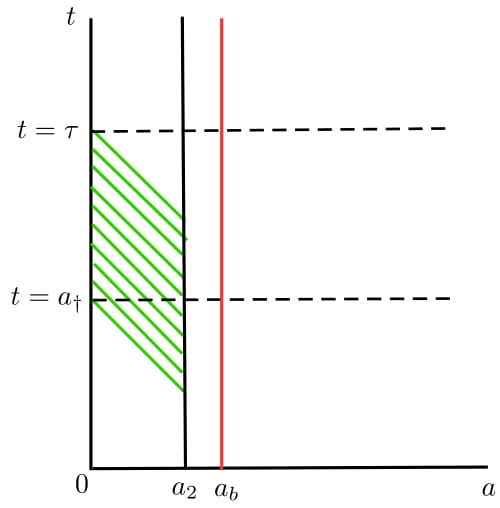 Fig.1 - An ilustration of the estimate of $q(t,0).$ We apply final state observability of $(A^*, B^*)$ along
the characteristics. Since we want to estimate $q(t,0),$ we consider the trajectory $\gamma(s) = (t-s,s),$
$s \leqslant t \leqslant \tau$ (or equivalently the backward characteristics starting from $(t,0).$)
Fig.1 - An ilustration of the estimate of $q(t,0).$ We apply final state observability of $(A^*, B^*)$ along
the characteristics. Since we want to estimate $q(t,0),$ we consider the trajectory $\gamma(s) = (t-s,s),$
$s \leqslant t \leqslant \tau$ (or equivalently the backward characteristics starting from $(t,0).$)
|
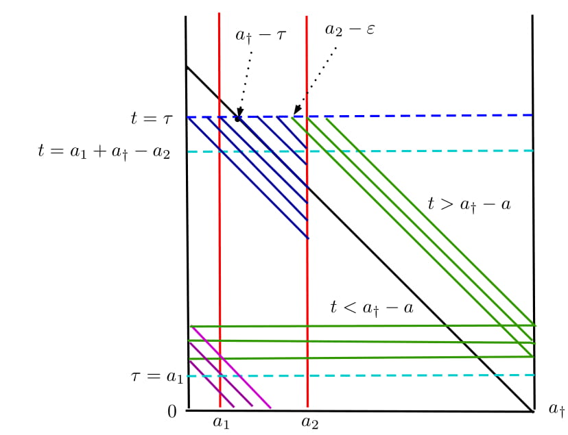 Fig.2 - An illustration of the final-state observability at time $\tau > a_1 + a_\dagger - a_2$: For
$ a \in (0,a_2 - \varepsilon)$ (blue region) the backward characteristics starting from $t = \tau$ enters the
observation domain. For $a \in (a_2 - \varepsilon, a_\dagger)$, the backward characteristics (green region)
hits the line $a = a_\dagger$, gets renewed by the renewal condition $\beta(a)q(t,0)$ and then enters the observation
domain (purple region).
Fig.2 - An illustration of the final-state observability at time $\tau > a_1 + a_\dagger - a_2$: For
$ a \in (0,a_2 - \varepsilon)$ (blue region) the backward characteristics starting from $t = \tau$ enters the
observation domain. For $a \in (a_2 - \varepsilon, a_\dagger)$, the backward characteristics (green region)
hits the line $a = a_\dagger$, gets renewed by the renewal condition $\beta(a)q(t,0)$ and then enters the observation
domain (purple region).
|
Examples
We consider two examples : 1) The classical Lotka-McKendrick system and 2) Lotka-Mckendrick system with diffusion.
1) The classical Lotka-McKendrick system : Let us choose $X = \mathbb{R},$ $A=0$ and $B=1.$ Then the system \eqref{eq:main} reduces
to classical Lotka-McKendrick system. By Theorem 1, this system is null controllable in time $\tau > a_1 + a_\dagger - a_2.$ A
similar result was obtained in [1].
2) The Lotka-McKendrick system with spatial diffusion : Let $\Omega$ be a smooth bounded domain in $\mathbb{R}^3$ and
$\omega \subseteq \Omega.$ Let us consider
\begin{equation*}
X = L^2(\Omega), \quad A = \Delta , \quad \mathcal{D}(A) =
\left\{ f \in H^2(\Omega) \mid \displaystyle \frac{\partial f}{\partial n} = 0\right\}, \quad B = \chi_{\omega}.
\end{equation*}
This corresponds to the Lotka-McKendrick model with spatial diffusion ([2]). It is known that, the pair $(A, B)$ or equivalently
the heat equation with localized interior control, is null controllable in any time. Thus we can apply Theorem 1 to conclude that
the system is null controllable in time $\tau > a_1 + a_\dagger - a_2.$
Several other applications can be found in [3].
Numerical Simulations
We now present some numerical siimulations of the controlled trajectory. We shall consider the case $A = 0$
and $B = 1,$ i.e the classical Lotka-McKendrick system. We also consider the case $a_1 = 0$ and $a_2 = a_{\dagger} =4,$ i.e., the control
acts everywhere with respect to age variable. We present numerical simulations in the following two scenarios : 1) null controllabilty,
2) controllability to a steady state.
Null Controllability
By Theorem 1 we know that system (1) is null controllable in any time. In the following
video, we see the evolution of unctrolled trajectory and controlled trajectories to zero with controllability time $t=2$ and $t =5.$
We now plot the control functions. In the following two videoes, we see the evolution of the control
functions at controllability time $t = 2$ and $t =5$
respectively.
Controllability to a steady state
If we choose $\beta$ and $\mu$ such that $R = \int_0^{a_\dagger} \beta(a) e^{-\int_0^r \mu(r) \ dr } da = 1,$ then
$p_s(a) = \alpha e^{-\int_0^r \mu(r) \ dr }$ with $\alpha \in (0,\infty)$ is a steady state to the system (1) with zero steady control.
Thus we can control to these trajectories also. In the following example, we have chosen $a_{\dagger} = 4,$ $a_b = 1,$ $\alpha = 1.25$ and
\begin{equation*}
\beta(a) = \begin{cases}
0 & \mbox{ if } a \in [0,1), \\
\frac{1}{3}e^{.05 a^2} & \mbox{ if } a \in [1,4],
\end{cases}
\qquad
\mu(a) = .1 a.
\end{equation*}
In this case we can verify that $R=1$ and $p_s(a) = 1.25 e^{-.05 a^2}.$ As before we take control everywhere, thus the system is
controllable to the trajectory $p_s(a)$ in any time. In the following video,
we see the evolution of unctrolled trajectory and controlled trajectories to the steady state $p_s(a)$ with
controllability time $t=2$ and $t =5.$
As before, in the following two videos we see the evolution of the control functions at time $t =2$ and $t=5$ respectively.
References
[1] D. Maity, On the Null Controllability of the Lotka-Mckendrick System, Submitted.
[2] D. Maity, M. Tucsnak and E. Zuazua, Controllability and positivity constraints in population dynamics with age
structuring and diffusion , Journal de Mathématiques Pures et Appliqués. In press, 10.1016/j.matpur.2018.12.006.
[3] D. Maity, M. Tucsnak and E. Zuazua, Controllability of a Class of Infinite Dimensional
Systems with Age Structure. Submitted.
[4] M. Tucsnak and G. Weiss, Observation and control for operator semigroups,
Birkhäuser Advanced Texts: Basler Lehrbuücher. [Birkhäuser Advanced Texts: Basel Textbooks], Birkhäuser Verlag, Basel, 2009.