Download Code
It is superfluous to state the impact deep learning has had on modern technology. From a mathematical point of view however, a large number of the employed models remain rather ad hoc.
When formulated mathematically, deep supervised learning roughly consists in solving an optimal control problem subject to a nonlinear discrete-time dynamical system, called an artificial neural network.
1. Setup
Deep supervised learning [1, 3] (and more generally, supervised machine learning), can be summarized by the following scheme.
We are interested in approximating a function $f: \R^d \rightarrow \R^m$, of some class, which is unknown a priori. We have data: its values
at $S$ distinct points (possibly noisy).
We generally split the $S$ data points into training data and testing data . In practice, $N\gg S-N-1$.
“Learning” generally consists in:
- Proposing a candidate approximation
$f_\Theta( \cdot): \R^d \rightarrow \R^m$, depending on tunable parameters $\Theta$ and fixed hyper-parameters $L\geq 1$, ${ d_k}$;
-
Tune $\Theta$ as to minimize the empirical risk:
where $\ell \geq 0$, $\ell(x, x) = 0$ (e.g. $\ell(x, y) = |x-y|^2$). This is called training.
- A posteriori analysis: check if test error is small.
This is called generalization.
Remark:
-
There are two types of tasks in supervised learning:
classification ($\vec{y}_i \in {-1,1}^m$ or more generally, a discrete set), and regression ($\vec{y}_i \in \R^m$).
We will henceforth only present examples of binary classification, namely $\vec{y}_i \in {-1, 1}$, for simple presentation purposes.
-
Point 3 is inherently linked with the size of the control parameters $\Theta$.
Namely, a penalisation of the empirical risk in theory provides better generalisation.
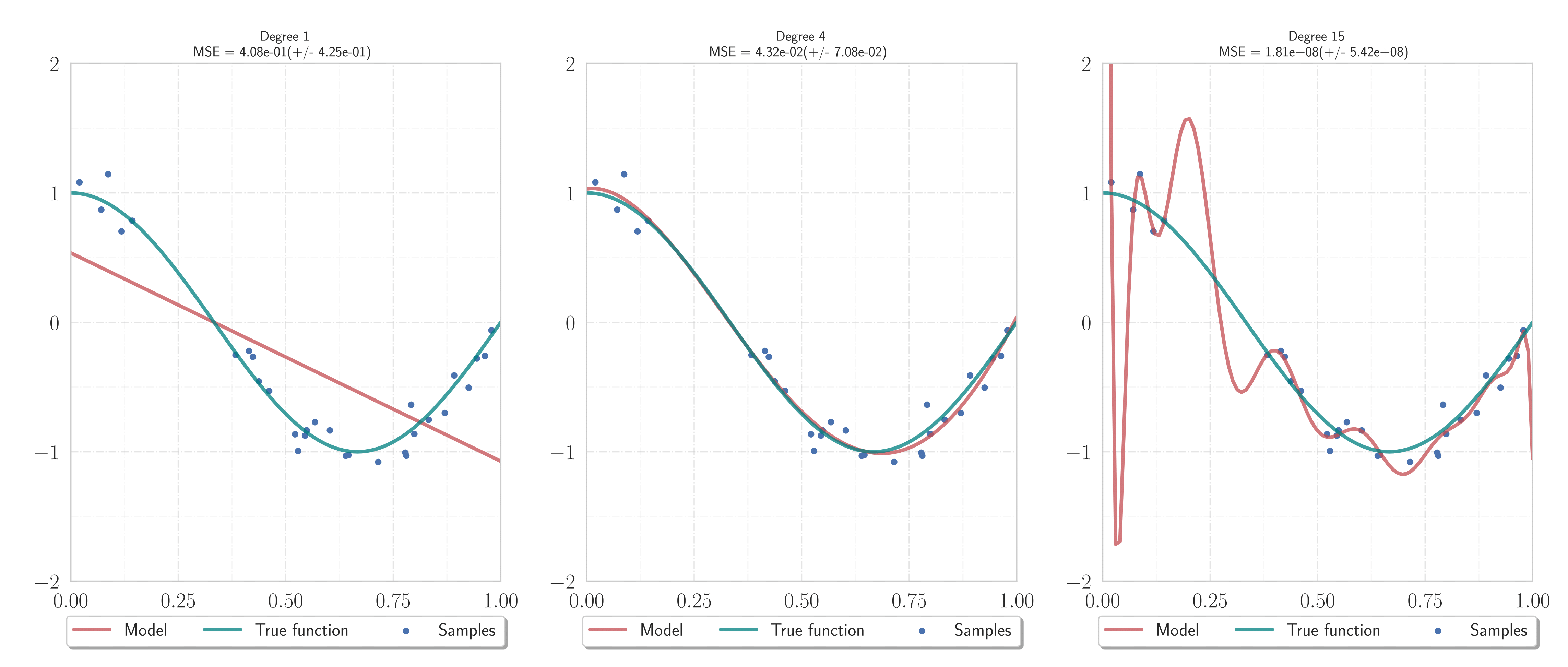 Figure 1.
Underfitting, good generalization, and overfitting. We wish to recover the function $f(x) = \cos(\frac32 \pi x)$ (blue) on $(0, 1)$ from $S=20$ noisy data samples.
Constructed approximations using $N=12$ training data, while the remaining $8$ samples are used for testing the results. The most complicated model (right) is not necessarily the best (Occam's razor).
This is related to the Runge phenomenon.
Figure 1.
Underfitting, good generalization, and overfitting. We wish to recover the function $f(x) = \cos(\frac32 \pi x)$ (blue) on $(0, 1)$ from $S=20$ noisy data samples.
Constructed approximations using $N=12$ training data, while the remaining $8$ samples are used for testing the results. The most complicated model (right) is not necessarily the best (Occam's razor).
This is related to the Runge phenomenon.
Remark: It is at the point of generalisation where the objective of supervised learning differs slightly from classical optimisation/optimal control. Indeed, whilst in deep learning one too is interested in “matching” the labels $\vec{y}_i$ of the training set, one also needs to guarantee satisfactory performance on points oustide of the training set.
2. Artificial Neural Networks
There exists an entire jungle (see [1, 3]) of specific neural networks used in practice and studied in theory.
For the sake of presentation, we will discuss two of the most simple examples.
2.1. Multi-layer perceptron
We henceforth assume that we are given a training dataset
.
Definition (Neural network): Let and be given. Set $d_0 := d$ and $d_{L+1} :=m$.
A neural network with $L$ hidden layers is a map
where $z^L = z^L_i \in \R^m$ being given by the scheme
Here are given parameters such that $A^k \in \R^{d_{k+1}\times d_k}$ and $b^k \in \R^{d_k}$, and $\sigma \in C^{0, 1}(\R)$ is a fixed, non-decreasing function.
Remark: Several remarks are in order:
- The above-defined neural network is usually referred to as the multi-layer perceptron (see Multilayer_perceptron)
- Observe that $z^k \in \R^{d_k}$ for .
- The function $\sigma$ is always nonlinear in practice (as otherwise the optimisation problem roughly coincides with least squares for a linear regression). It is called the activation function.
- Generally, $\sigma(x) = \max(x, 0)$ or $\sigma(x) = \tanh(x)$ (but others work too).
- Deep learning means optimisation subject to a multi-layered neural net: $L\geq 2$ at least.
Let us denote $\Lambda_k x :=A^k x + b^k$.
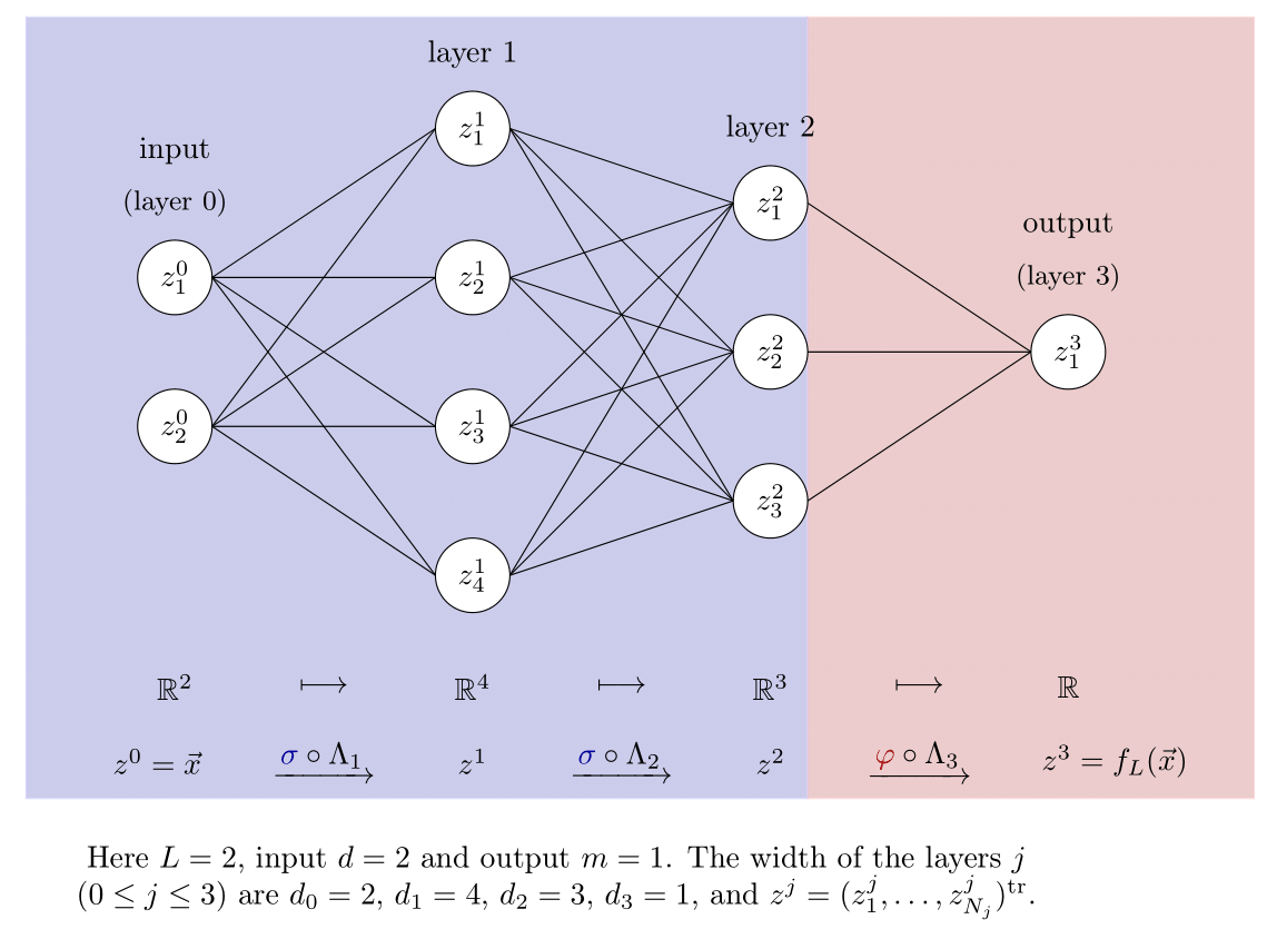 Figure 2.
The commonly used graph representation for a neural net.
This figure essentially represents the discrete-time dynamics of a single datum from the training set through the nonlinear scheme.
Figure 2.
The commonly used graph representation for a neural net.
This figure essentially represents the discrete-time dynamics of a single datum from the training set through the nonlinear scheme.
An MLP scheme with $\sigma(x) = \tanh(x)$ can be coded in pytorch more or less as follows:
import torch.nn as nn

class OneBlock(nn.Module):
	def __init__(self, d1, d2):
		super(OneBlock, self).__init__()
		self.d1 = d1
		self.d2 = d2

		self.mlp = nn.Sequential(
			nn.Linear(d1, d2),
			nn.Tanh()
		)
	def forward(self, x):
		return self.mlp(x)

class Perceptron(nn.Module):
	def __init__(self, dimensions, num_layers):
		super(Perceptron, self).__init__()

		self.dimensions = dimensions
		_ = \
			[OneBlock(self.dimensions[k], self.dimensions[k-1]) for k in range(1, num_layers-1)]

		self.blocks = nn.Sequential(*_)
		self.projector = nn.Linear(self.dimensions[-2], self.dimensions[-1])

	def forward(self, x)_
		return self.projector(self.blocks(x))
We can save this class in a file called model.py.
Then one may create an instance of a Perceptron model for practical usage as follows:
import torch
device = torch.device('cpu')
from model import Perceptron

model = Perceptron(device, dimensions=[1,3,4,3,1], num_layers=5)
How it works.
We now see, in some overly-simplified scenarios, how the forward propagation of the inputs in the context of binary classification.
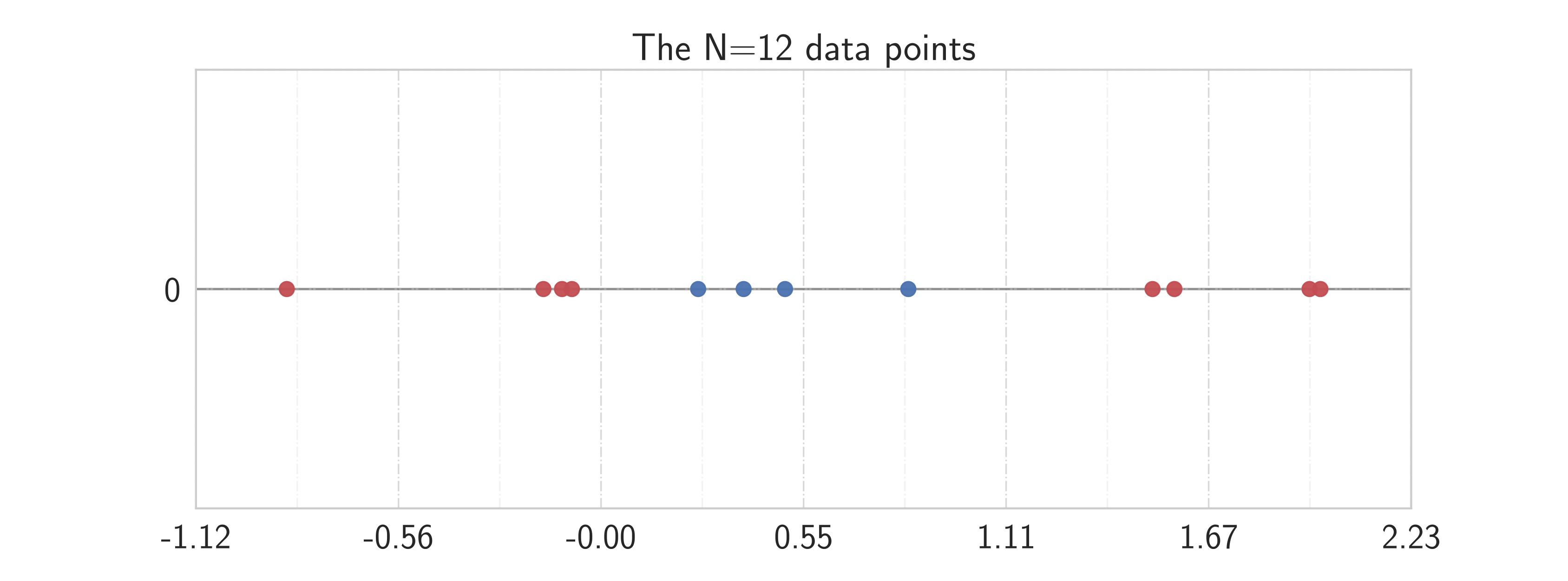 Figure 3.
Here $A^0 \in R^{2\times 1}$ and $b^0 \in \R^2$.
We see how the neural net essentially generates a nonlinear transform, such that the originally mixed points are now linearly separable.
Figure 3.
Here $A^0 \in R^{2\times 1}$ and $b^0 \in \R^2$.
We see how the neural net essentially generates a nonlinear transform, such that the originally mixed points are now linearly separable.
An interesting blog on visualising the transitions is the following: https://colah.github.io/posts/2014-03-NN-Manifolds-Topology/.
2.2. Residual neural networks
We now impose that the dimensions of the iterations and the parameters stay fixed over each step.
This will allow us to add an addendum term in the scheme.
Definition (Residual neural network [2]): Let and be given. Set $d_0 := d$ and $d_{L+1} :=m$.
A residual neural network (ResNet) with $L$ hidden layers is a map
where $z^L = z^L_i \in \R^d$ being given by the scheme
Here $\Theta = {A^k, b^k}_{k=0}^{L}$ are given parameters such that $A^k \in \R^{d\times d}$ and $b^k \in \R^{d}$ for $k<L$ and $A^L \in \R^{m\times d}, b^L \in \R^m$, and $\sigma \in C^{0, 1}(\R)$ is a fixed, non-decreasing function.
3. Training
Training consists in solving the optimization problem:
- $\epsilon>0$ is a penalization parameter.
- It is a non-convex optimization problem because of the non-linearity of $f_L$.
- Existence of a minimizer may be shown by the direct method.
Once training is done, and we have a minimizer $\widehat{\Theta}$, we consider $f_{\widehat{\Theta}}(\cdot)$ and use it on other points of interest $\vec{x} \in \R^d$ outside the training set.
3.1. Computing the minimizer
The functional to be minimized is of the form
We could do gradient descent:
$\eta$ is step-size. But often $N \gg 1$ ($N=10^3$ or much more).
Stochastic gradient descent: (Robbins-Monro [7], Bottou et al [8]):
-
pick $i \in {1, \ldots, N}$ uniformly at random
-
$\Theta^{n+1} := \Theta^n - \eta \nabla J_{i}(\Theta^n)$
- Mini-batch GD: can also be considered (pick a subset of data instead of just one point)
- Use chain rule and adjoints to compute these gradients (“backpropagation”)
- Issues: might not converge to global minimizer; also how does one initialize the weights in the iteration (usually done at random)?
We come back to the file model.py. Here is a snippet on how to call training modules.
# Given generated data
# Coded a function def optimize() witin
# a class Trainer() which
# does the optimization of paramterss

epochs = input()
optimizer = torch.optim.SGD(perceptron.parameters(), lr=1e-3, weight_decay=1e-3)

trainer = Trainer(perceptron, optimizer, device)
trainer.train(data, epochs)
3.2. Continuous-time optimal control problem
We begin by visualising how the flow map of a continuous-time neural net separates the training data in a linear fashion at time $1$ (even before in fact).
Figure 4.
The time-steps play the role of layers. We are working with an ode on $(0, 1)$. We see that the points are linearly separable at the final time, so the flow map defines a "linearisation" of the training dataset.
Recall that often $\varphi \equiv \sigma$ (classification) or $\varphi(x) = x$ (regression).
It can be advantageous to consider the continuous-time optimal control problem:
where $z = z_i$ solves
Remark:
The ResNet neural network can then be seen as the forward Euler discretisation with $\Delta t = 1$.
The relevance of this scale when passing from continuous to discrete has not been addressed in the litearature.
Thus, in the continuous-time limit, deep supervised learning for ResNets can be seen as an optimal control problem for a parametrised, high-dimensional ODE.
This idea of viewing deep learning as finite dimensional optimal control was (mathematically) formulated in [12], and subsequently investigated from a theoretical and computational viewpoint in [11, 10, 5, 6, 13, 14], among others.
Remark:
There are many tricks which can be used in the above ODE to improve performance.
- For instance, we may embed the initial data in a higher dimensional space at the beginning, and consider the system in an even bigger dimension. It is rather intuitive that the bigger the dimension where the system evolves is, the easier it is to separate the points by a hyperplane.
- However, characterising the optimal dimension where one needs to consider the evolution of the neural net in terms of the topology of the training data is, up to the best of our knowledge, an open problem.
The choice in practice is done by cross-validation.
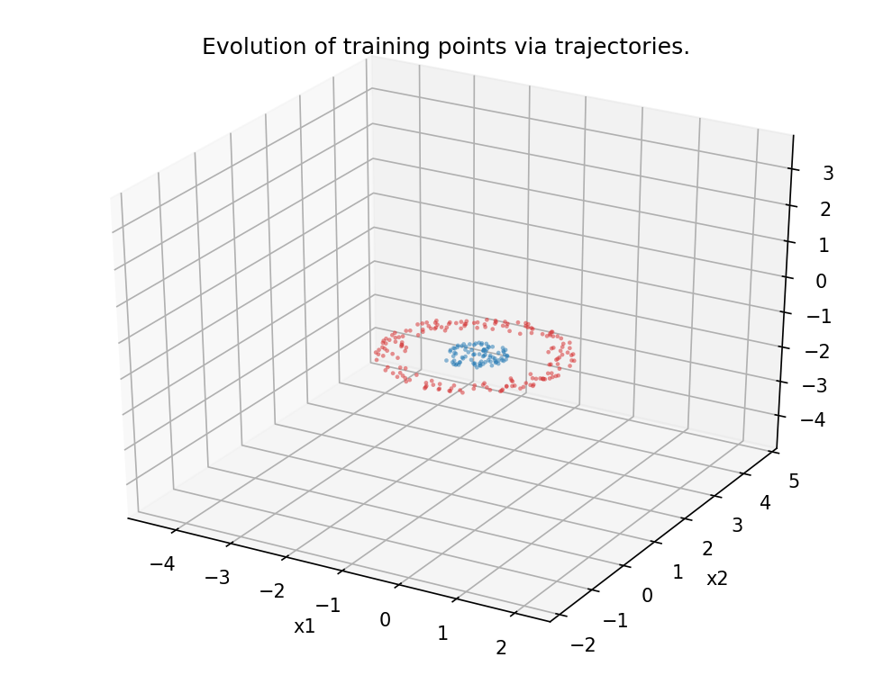 Figure 5.
Analogous scenario as in Figure 4, this time in dimension 3.
Figure 5.
Analogous scenario as in Figure 4, this time in dimension 3.
References:
[1] Ian Goodfellow and Yoshua Bengio and Aaron Courville. (2016). Deep Learning, MIT Press.
[2] He, K., Zhang, X., Ren, S., and Sun, J. (2016). Deep residual learning for image
recognition. In Proceedings of the IEEE conference on computer vision and pattern recognition, pages
770–778.
[3] LeCun, Y., Bengio, Y., and Hinton, G. (2015). Deep learning. Nature,
521(7553):436–444.
[4] LeCun, Y., Boser, B. E., Denker, J. S., Henderson, D., Howard, R. E., Hubbard,
W. E., and Jackel, L. D. (1990). Handwritten digit recognition with a back-propagation network. In
Advances in neural information processing systems, pages 396–404.
[5] Chen, T. Q., Rubanova, Y., Bettencourt, J., and Duvenaud, D. K. (2018). Neural
ordinary differential equations. In Advances in neural information processing systems, pages 6571–
6583.
[6] Dupont, E., Doucet, A., and Teh, Y. W. (2019). Augmented neural odes. In
Advances in Neural Information Processing Systems, pages 3134–3144.
[7] Herbert Robbins and Sutton Monro. A Stochastic Approximation Method. The Annals of Mathematical Statistics, 22(3):400–407, 1951
[8] Léon Bottou, Frank E. Curtis and Jorge Nocedal: Optimization Methods for Large-Scale Machine Learning, Siam Review, 60(2):223-311, 2018.
[9] Matthew Thorpe and Yves van Gennip. Deep limits of residual neural networks. arXiv preprint arXiv:1810.11741, 2018.
[10] Weinan, E., Han, J., and Li, Q. (2019). A mean-field optimal control formulation
of deep learning. Research in the Mathematical Sciences, 6(1):10.
[11] Li, Q., Chen, L., Tai, C., and Weinan, E. (2017). Maximum principle based algorithms
for deep learning. The Journal of Machine Learning Research, 18(1):5998–6026.
[12] Weinan, E. (2017). A proposal on machine learning via dynamical systems. Communications in Mathematics and Statistics, 5(1):1–11.