Download Code
The finite-dimensional dynamical system given by a pendulum on a cart (cartpole) is widely considered as a benchmark for comparing the performance of different control strategies. In this blog post, we consider a double pendulum on a cart and we solve the problem of swinging up the pendulum from the downward position to the upward position using optimal control techniques.
Setup
In this tutorial we need DyCon Toolbox, to install it we will have to write the following in our MATLAB console:
unzip('https://github.com/DeustoTech/DyCon-Computational-Platform/archive/master.zip')
addpath(genpath(fullfile(cd,'DyCon-toolbox-master')))
StartDyConToolbox
You can see the code of this tutorial write the following line:
open T06ODET0006_Double_pend
Equations of motion
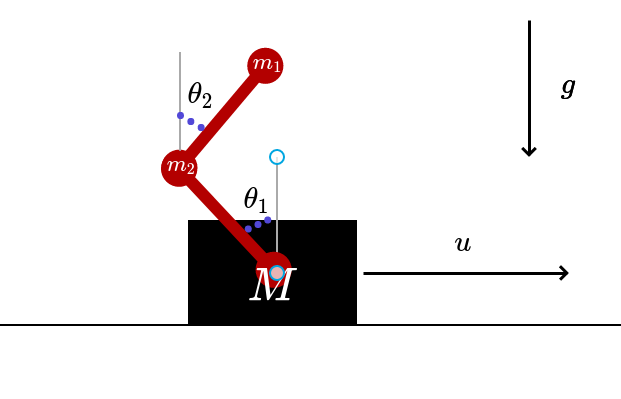
Figure 1. Scheme of system dynamics
The physical system defined by the double pendulum in a cart can be modelled as a system of six ordinary differential equations, whose state at each instant of time $t \geq 0$ is the vector $y(t) = \left( x(t), \theta_{1}(t), \theta_{2}(t), v(t), \omega_{1}(t), \omega_{2}(t) \right)$, where:
- $x(t) \in \mathbb{R}$ is the position of the cart.
- $\theta_{i}(t) \in [0, 2\pi]$ is the angle of the $i$-th pendulum.
- $v(t) \in \mathbb{R}$ is the velocity of the cart.
- $\omega_{i}(t) \in \mathbb{R}$ is the angular velocity of the $i$-th pendulum.
The equations of motion of the system can be derived using the Lagrangian formalism of classical mechanics and are given by:
where, for each $t \geq 0$, we define:
and
We have the fixed parameters:
- $d_{i} \in [0,1]$ are damping coefficients.
- $m > 0$ is the mass of the cart and $m_{i} > 0$ is the mass of the $i$-th pendulum.
- $l_{i} > 0$ is the length of the $i$-th pendulum.
The function $u \in L^{\infty}(0,\infty; \mathbb{R})$ is a time-dependent control that acts on the acceleration term $\dot{v}(t)$ of the cart, and can thus be interpreted as a force that is exerted on the cart.
This dynamical system shows chaotic behaviour. The following animation displays the evolution of the double pendulum on a cart with control $u = 0$ and starting at the two different initial conditions
Figure 2. Chaotics behaviour
Optimal Control Problem
We will solve the problem of steering the state of the pendulum from the downward position $y_{0} = (0, \pi, \pi, 0, 0, 0)$ to the upward position $z = (0, 0, 0, 0, 0, 0)$ in a fixed time horizon $T > 0$ using a control $u(t)$.
One way to look for solutions to this problem is to minimize the following functional:
Where $\alpha >0$ is a fixed parameter, the state vector $y(t)$ is subject to the system of differential equations (1) and $y(0) = y_0$.
Numerical simulation
We start by implementing the dynamical system defined in (1) as a MATLAB function. We fix the lengths $l_{i} = 1$, and the mass of the cart $M = 50$. The damping coefficients are set to $d_{i} = 0.1$.
  >> type cartpole_dynamics.m

function ds = cartpole_dynamics(t,s,u,params)
    L1 = 1;    L2 = 1;    g = 9.8;
    m1 = params.m1;    m2 = params.m2;
    M = 50;
    d1 = 1e-1;    d2 = 1e-1;    d3 = 1e-1;
    %%%%%%%%%%%%%%%%%%%%%5%%%
    ds = zeros(6,1,class(s));
    %
    q      = s(1);    theta1 = s(2);
    theta2 = s(3);    dq     = s(4);
    dtheta1= s(5);    dtheta2= s(6);
    % q
    ds(1) = dq -q;
    % theta 1
    ds(2) = dtheta1;
    % theta 2
    ds(3) = dtheta2;
    %
    Mt = [ M+m1+m2                  L1*(m1+m2)*cos(theta1)     m2*L2*cos(theta2) ; ...
          L1*(m1+m2)*cos(theta1)     L1^2*(m1+m2)             L1*L2*m2*cos(theta1-theta2) ; ...
          L2*m2*cos(theta2)          L1*L2*m2*cos(theta1-theta2)  L2^2*m2        ];
    % v
    f1 = L1*(m1+m2)*dtheta1^2*sin(theta1) + m2*L2*theta2^2*sin(theta2)      - d1*dq + u  ;
    f2 = -L1*L2*m2*dtheta2^2*sin(theta1-theta2) + g*(m1+m2)*L1*sin(theta1)  - d2*dtheta1;
    f3 =  L1*L2*m2*dtheta1^2*sin(theta1-theta2) + g*L2*m2*sin(theta2)       - d3*dtheta2;

    ds(4:6) = Mt\[f1;f2;f3];
end
This optimal control problem is solved using CasADi with the IPOPT solver. MATLAB’s symbolic toolbox has been used to implement the system dynamics in CasADi.
The time horizon is set to $T = 10$ and the system (1) has been discretized using a Crank-Nicolson scheme. The use of an implicit discretization method with good behaviour with respect to the number of mesh points has been crucial to speed up the optimization process.
import casadi.*
% define optimal

Ss = SX.sym('x',6,1);As = SX.sym('u',1,1);ts = SX.sym('t');
%
EvolutionFcn =  cartpole_dynamics(ts,Ss,As,params) ;
%
dynamics_obj = ode(EvolutionFcn,ts,Ss,As,tspan);
dynamics_obj.InitialCondition = s0;
%
PathCost  =  (Ss.'*Ss) + 1e-5*(As.'*As) ;
FinalCost = (Ss.'*Ss ) ;

ocp_obj = ocp(dynamics_obj,PathCost,FinalCost);
%
U0 =0*tspan;
[OptControl ,OptState] = IpoptSolver(ocp_obj,U0,'integrator','CrankNicolson');
The following animation displays the resulting evolution of the system’s state:
Figure 3. Optimal solution
Interestingly, due to the chaotic character of system (1), the IPOPT routine yields different controlled trajectories if we change the initial guess of the control:
Figure 4. Several initial guess of optimization