Optimal Shape Design for Poisson Equation in Matlab

Download Code

We study the shape design problem through the minimization of the cost functional

$\mathcal{J} \left( \theta, y \right) = \frac{1}{2} \int_{\Omega \left( \theta \right )} \left( y - y_d \right) ^2 \, \mathrm{d} \Omega,$

where $y \in L^2 \left( \Omega \right)$ is the state variable, $y_d \in L^2 \left( \Omega \right)$ is a target function, and $\theta \left( \mathbf{x} \right)$ the normal displacement to a reference boundary,

$\Gamma \left( \theta \right) = \left\{ \mathbf{x} + \theta \left( \mathbf{x} \right) \mathbf{n} \left( \mathbf{x} \right) : \mathbf{x} \in \Gamma_{0} \right\}.$

The problem is subject to the following elliptic PDE in the domain $\Omega \left( \theta \right ) \subset \mathbb{R}^d$ with Dirichlet boundary conditions on $\Gamma \left( \theta \right ) = \Gamma_w \cup \Gamma_s \left( \theta \right )$ ,

$\begin{cases} -\Delta y = f & \text{in } \Omega \left( \theta \right ),\\ y = y_{w} & \text{in } \Gamma_w,\\ y = y_{s} & \text{in } \Gamma_s \left( \theta \right ), \end{cases}$

and $f \in L^2 \left( \Omega \right)$ .

We consider the set of admissible domains whose measure is fixed,

$\mathcal{U}_{ad} = \left\{ \Omega \left( \theta \right ) : \lvert \Omega \left( \theta \right ) \rvert = \Omega_0 \right\},$

and aim at finding the optimal shape that minimizes the cost function. In order to do so, we use the steepest descent method with descent direction given by

$\delta \theta ^{\left( n \right)} = - \left[ \frac{1}{2} \left( y^{\left( n \right)} - y_d \right) ^2 + \frac{\partial v}{\partial n}^{\left( n \right)} \frac{\partial y}{\partial n}^{\left( n \right)} + q^{\left( n \right)} \right],$

where $v$ is solution of the adjoint problem

$\begin{cases} - \Delta v = y - y_d & \text{in } \Omega \left( \theta \right ), \\ v = 0 & \text{on } \Gamma \left( \theta \right ) = \Gamma_w \cup \Gamma_s \left( \theta \right ). \end{cases}$

The normal displacement field is updated at every iteration,

$\theta^{\left( n + 1 \right)} = \theta^{\left( n \right)} + \epsilon \delta{\theta^{\left( n \right)}},$

with $\epsilon$ sufficiently small. The Lagrange multiplier is computed in order to ensure that the volume contraint is fulfilled, thus

$q^{\left( n \right)} = - \frac{1}{\left|\Gamma_s \left( \theta \right )\right|} \int_{\Gamma_s \left( \theta \right )} \left[ \frac{1}{2} \left( y^{\left( n \right)} - y_d \right) ^2 + \frac{\partial v}{\partial n}^{\left( n \right)} \frac{\partial y}{\partial n}^{\left( n \right)} \right] \mathrm{d} \Gamma.$

Mesh Motion Solver

The solutions to the primal and adjoint problems are commonly approximated by means of numerical methods, such as the finite element method (FEM) or the finite volume method (FVM). In order to apply these techniques, the domain under study must be tessellated with a mesh. Nevertheless, applying the displacement directly to the controlled boundary will deteriorate the surrounding elements after a few iterations and the computation will crash if the interior nodes of the domain are not reallocated. In order to avoid this, the domain can be re-meshed after a number of iterations. However, this can be very expensive as a completely new mesh must be generated. A commonly used alternative is to move the interior nodes of the mesh according to the displacements prescribed on the boundary. By doing this the number of elements and the nodes connectivities remain the same, only the mesh nodes positions are updated.

Linear Elasticity

Mesh motion can be achieved by treating the mesh as an elastic body and solving the equations of Linear Elasticity for solids with prescribed displacements on the domain boundary,

$\begin{cases} \partial_j \left( G \partial_j u_i \right) + \partial_j \left( G \partial_i u_j \right) + \partial_i \left( \lambda \partial_j u_j \right) = 0 & \text{in } \Omega \left( \theta \right ), \\ u_i = 0 & \text{on } \Gamma_w, \\ u_i = \delta \theta n_i & \text{on } \Gamma_s \left( \theta \right ). \end{cases}$

Solid Body Rotation (SBR) Stress

The Linear Elasticity model fails when dealing with rotating meshes. This can be mitigated by selecting the material properties in a proper manner, which yields

$\begin{cases} 2 \partial_j \left( \gamma \left( \mathbf{x} \right) \partial_j u_i \right) + \partial_j \left[ \gamma \left( \mathbf{x} \right) \left( \partial_i u_j - \partial_j u_i - \delta_{ij} \partial_k u_k \right) \right] = 0, & \text{in } \Omega \left( \theta \right ), \\ u_i = 0 & \text{on } \Gamma_w, \\ u_i = \delta \theta n_i & \text{on } \Gamma_s \left( \theta \right ). \end{cases}$

Laplacian Smoothing

A simple and widely used practice is to solve a Laplace equation with the prescribed displacements as boundary conditions,

$\begin{cases} \Delta u_i = 0 & \text{in } \Omega \left( \theta \right ), \\ u_i = 0 & \text{on } \Gamma_w, \\ u_i = \delta \theta n_i & \text{on } \Gamma_s \left( \theta \right ). \end{cases}$

The behavior of the Laplacian smoothing can be improved by adding a non-uniform diffusivity term,

$\partial_k \left( \gamma \left( \mathbf{x} \right) \partial_k u_i \right) = 0 \quad \text{in } \Omega \left( \theta \right ).$

The diffusion field $\gamma \left( \mathbf{x} \right): \mathbb{R}^d \rightarrow \mathbb{R}$ decreases with the distance to the controlled boundary. A common choice is to make it depend on the inverse of the distance as

$\gamma \left( \mathbf{x} \right) = \frac{1}{d^m},$

so that the nodes next to the deforming boundaries move with similar displacements as those on the boundary.

Spring Analogy

A more intuitive approach is reached by thinking of the N mesh nodes as a mechanical system consisting of a finite set of masses that are linked with springs along the mesh edges. We can consider the existence of additional external forces acting on every mesh node, so that for every equilibrium configuration the following must hold,

$\mathbf{F}_i - \sum_{j=1}^N k_{ij} \left( \mathbf{x}_i - \mathbf{x}_j \right) = 0, \quad 1 \leq i \leq N.$

The equilibrium equations can be expressed in terms of the nodes displacements,

$\mathbf{\Delta F}_i - \sum_{j=1}^N k_{ij} \left( \mathbf{u}_i - \mathbf{u}_j \right) = 0, \quad 1 \leq i \leq N.$

At the M nodes that belong to the domain boundary the displacements are prescribed with unknown forces acting on them. On the other hand, on the interior nodes of the mesh whose displacements are unknown, there are no other forces than the elastic ones. Let us denote with D the indices of the nodes with prescribed displacement, and with S the set of nodes with unknown displacements. The equilibrium can be expressed in matrix form as

$\begin{align*} \mathbf{K}_{DD} \mathbf{u}_D + \mathbf{K}_{DS} \mathbf{u}_{S} & = \mathbf{\Delta F}_{D}, \\ \mathbf{K}_{SD} \mathbf{u}_D + \mathbf{K}_{SS} \mathbf{u}_{S} & = \mathbf{\Delta F}_{S} = \mathbf{0}. \end{align*}$

One can get the displacements of the interior mesh nodes as

$\mathbf{u}_S = -\mathbf{K}_{SS}^{-1} \mathbf{K}_{SD} \mathbf{u}_D.$

Radial Basis Functions (RBF)

The RBF mesh morphing technique uses the known displacements at the domain boundaries to construct an interpolation expression as a weighted sum of radial functions $\varphi: \mathbb{R} \rightarrow \mathbb{R}$ ,

$s^{\alpha} \left( \mathbf{x} \right) = \sum_{j=1}^N \gamma^{\alpha}_j \varphi \left( \| \mathbf{x} - \mathbf{x}_{s, j} \|_{\mathbb{R}^d} \right) + p^{\alpha} \left( \mathbf{x} \right), \quad 1 \leq \alpha \leq d.$

The weighting coefficients and the polynomials are obtained by imposing the known displacements at the boundaries,

$s^{\alpha} \left( \mathbf{x}_{s, i} \right) = g^{\alpha}_{s, i} = \delta \theta n^{\alpha},$

and the orthogonality conditions for every polynomial with degree less or equal than that of $p^{\alpha}$ ,

$\sum_{j=1}^N \gamma^{\alpha}_j q \left( \mathbf{x}_{s,j} \right) = 0, \quad 1 \leq \alpha \leq d.$

At the end, a linear system of the form

$\begin{pmatrix} \mathbf{M}_s & \mathbf{P}_s \\ \mathbf{P}_s^T & \mathbf{0} \end{pmatrix} \begin{pmatrix} \mathbf{\gamma}^{\alpha} \\ \mathbf{\beta}^{\alpha} \end{pmatrix} = \begin{pmatrix} \mathbf{g}_s^{\alpha} \\ \mathbf{0} \end{pmatrix}$

must be solved, and the mesh nodes are updated as

$x^{\mathrm{new}, \alpha} = x^{\mathrm{old}, \alpha} + s^{\alpha}\left( \mathbf{x}^{\mathrm{old}} \right).$

Free Form Deformation (FFD)

An alternative is to use some parametrization technique for the boundary $\Gamma_s \left( \theta \right )$ and extend it to be able to handle the motion of the interior nodes of the mesh as well. This can be done with the Free Form Deformation method, that is based upon the positions of a set of control points inside a parallelepiped.

If we consider the 2-dimensional reference control domain $\Omega_{st}=\left[ 0, 1 \right] \times \left[ 0 , 1 \right]$ , we can define a set of $\left( N + 1 \right) \times \left( M + 1 \right)$ evenly spaced control points,

$\mathbf{P}_{ij} = \left( \frac{i}{M}, \frac{j}{N} \right), \quad 0 \leq i \leq M, \quad 0 \leq j \leq N,$

and introduce the tensorial product of Bernstein polynomials $B_{ij}^{MN}\left[\mathbf{S} = \left(s, t \right) \right] = b_i ^M \left( s \right) b_j ^N \left( t \right)$ , with

$\begin{align*} b_i^M \left( s \right) &= \binom{M}{i} s^i \left(1-s\right) ^{M-i}, \\ b_j^N \left( t \right) &= \binom{N}{j} t^j \left(1-t\right) ^{N-j}. \end{align*}$

The transformation

$\mathbf{\Psi} \left( \mathbf{S} \right) = \sum_{i=0}^M \sum_{j=0}^N B_{ij}^{MN} \left( \mathbf{S} \right) \mathbf{P}_{ij}$

is the identity transformation, i.e., $\mathbf{\Psi}\left( \mathbf{S} \right) = \mathbf{S}$ .

We consider a set of control points defined as displacements from the reference positions, $\mathbf{P}_{ij} + \mathbf{\Delta P}_{ij}$ . In this case it is easy to see that the following holds

$\mathbf{ \Delta S } = \mathbf{ \Psi } \left( \mathbf{S} \right) - \mathbf{S} = \sum_{i=0}^M \sum_{j=0}^N B_{ij}^{MN} \left( \mathbf{S} \right) \mathbf{ \Delta P }_{ij}.$

We must find the control points displacements $\mathbf{\Delta P}_{ij} \in \Omega_{st}$ that parametrize the controlled boundary and for which, for every boundary node $\mathbf{X}_{s,k} \in \Gamma_s \left( \theta \right ), \ 1 \leq k \leq Z$ ,

$\mathbf{\Phi} \left( \mathbf{X}_{s,k} + \var{\theta} \mathbf{n} \right) - \mathbf{\Phi} \left( \mathbf{X}_{s,k} \right) = \sum_{i=0}^M \sum_{j=0}^N B_{ij}^{MN} \left[ \mathbf{\Phi} \left( \mathbf{X}_{s,k} \right) \right] \mathbf{ \Delta P}_{ij}, \quad 1 \leq k \leq M.$

Getting Started

The file main.m needs to be run from the Matlab command line,

main.m

Dynamic Mesh

The different mesh motion methods can be selected in the heading of main.m

%%%%%%%%%%%%%%%%%%%%%%%%%%%%%%%%%%%%%%%%%%%%%%%%%%%%%%%%%%%%%%%%%%%%%%%%%%%
% PARAMETERS
%%%%%%%%%%%%%%%%%%%%%%%%%%%%%%%%%%%%%%%%%%%%%%%%%%%%%%%%%%%%%%%%%%%%%%%%%%%
% Minimum element size
Hmin = 1e-3;
% Maximum elements size
Hmax = 0.05;
% Step theta^{n+1} = theta^{n} - d * Dtheta^{n}
d = 1e-3;
% Maximum number of iterations
maxIter = 2000000;
% Dirichlet boundary condition on the outer boundary
ue = 1;
% Dirichlet boundary condition on the inner boundary
uc = 0;
% Smoothing of sensitivity field
smoothing = true;
% Reshaping of elements whose edges are lying on the controlled boundary
reshaping = true;
% Mesh motion solver method:
% - Laplace Equation ('laplace')
% - Spring Analogy ('spring')
% - Free Form Deformation ('FFD')
% - Radial Basis Functions ('RBF')
meshMotionSolver = 'laplace';
% Parameters for Laplace method
% Diffusivity (diff)
% - Inverse distance ('invdist')
invdist = true;
m = 6;
% Parameters for FFD method:
% Mi - number of control points along X axis
% Nj - number of control points along Y axis
% Xmin, Xmax - coordinates defining the control rectangle
Mi = 9;
Nj = 9;
Xmin = [-0.7, -0.6];
Xmax = -Xmin;
% Parameters for RBF method
% h - Dimensionless radial distance (r/h)
% RBFtype - Radial Basis Functions
% - Spline type, n odd ('Rn')
% - Thin Plate Spline, n even ('TPSn')
% - Multiquadratic ('MQ')
% - Inverse multiquadratic ('IMQ')
% - Inverse quadratic ('IQ')
% - Gaussian ('GS')
% n - Exponent
h = 2.5*0.3;
RBFtype = 'R';
n = 1;

Running a Case

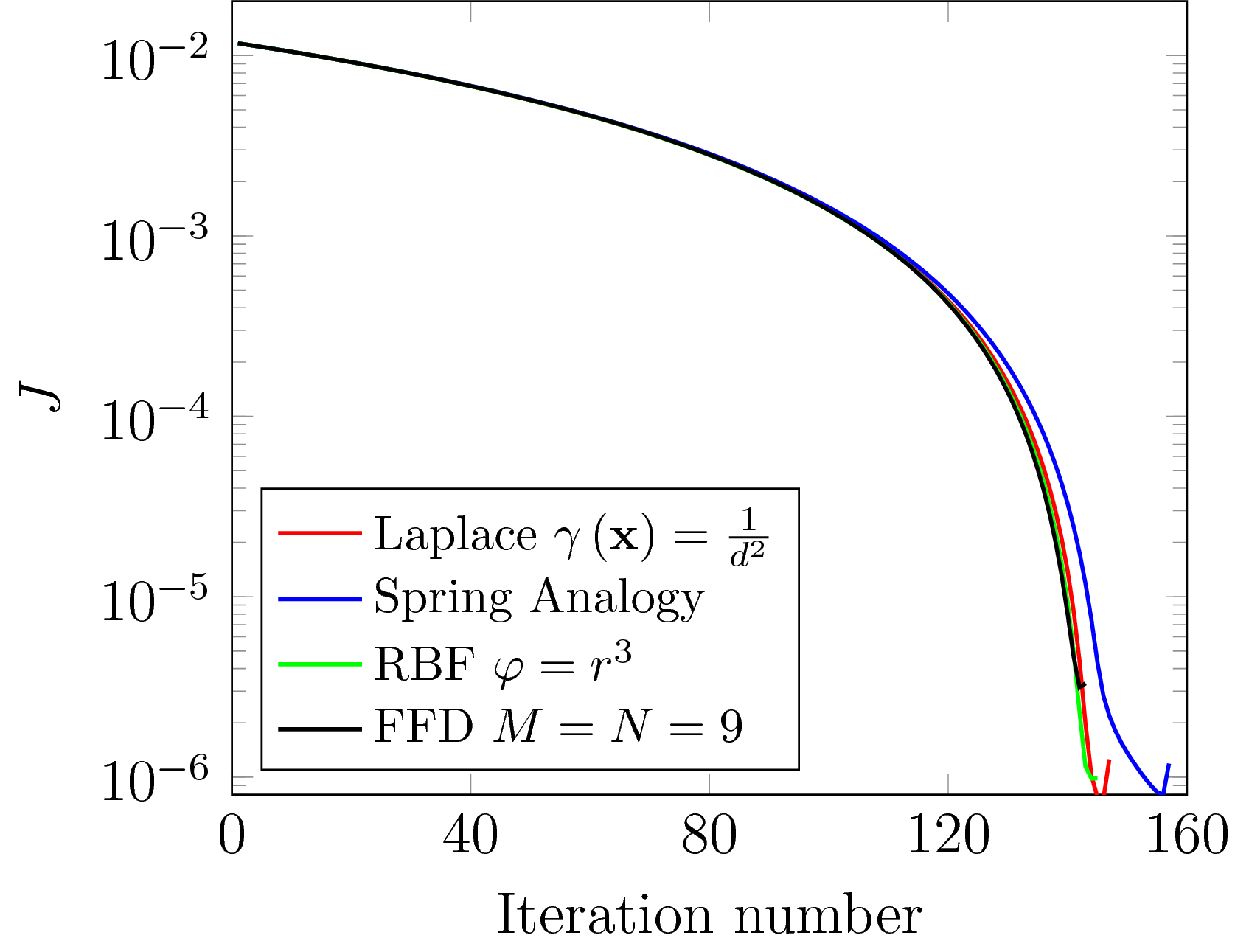
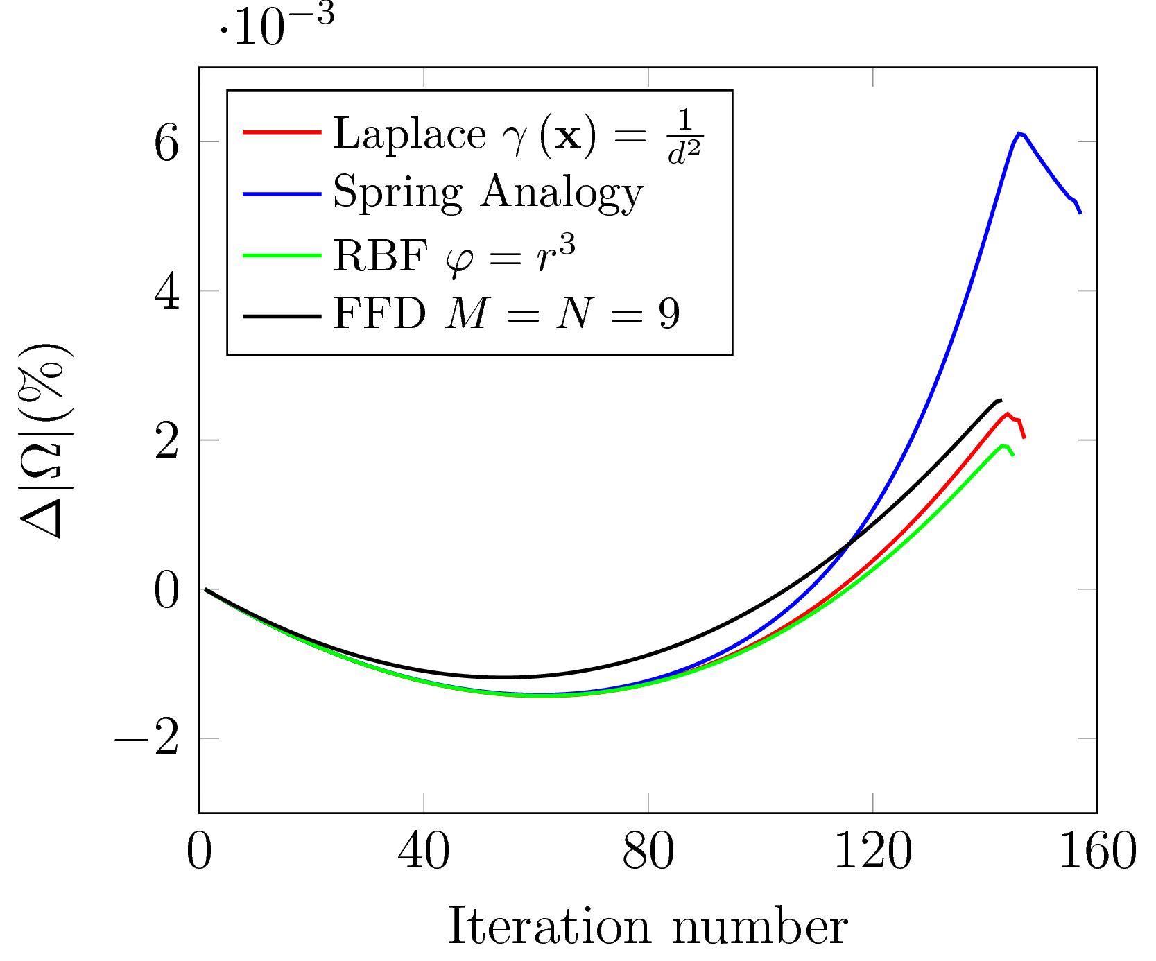
The shape optimization method described in the previous section has been tested with a simple example. The Poisson equation is posed in a two-dimensional circular domain with boundary

$\Gamma_w = \left\{ \left( x, y \right) \in \mathbb{R}^2: \sqrt{x^2 + y^2} = R_w \right\}.$

The reference geometry to be optimized is an inner hole with boundary given by

$\Gamma_s \left( 0\right) = \left\{ \left( x, y \right) \in \mathbb{R}^2 : \sqrt{\left( x - c_x \right)^2 + \left( y - c_y \right)^2} = R_s \right\}.$

The target function $u_d$ will be the analytical solution of the Poisson equation with the inner hole centered in the origin,

$u_{analytic}\left( r \right) = -\frac{f}{4}r^2 + c_1 \log r + c_2,$

where the integration constants are obtained from the boundary conditions,

$\begin{align*} c_1 = & \frac{u_w - u_s + \displaystyle \frac{f}{4} \left( R_w^2 - R_s^2 \right)}{\log\left( \displaystyle \frac{R_w}{R_s} \right)}, \\ c_2 = & \frac{u_w + u_s}{2} + \frac{f}{8}\left( R_w^2 + R_s^2 \right) - \frac{c_1}{2} \log\left( R_w R_s \right). \end{align*}$

When the hole center is displaced from the origin, the target state must be extended in the region $r \leq R_1$ , thus

$u_d\left( r \right)= \begin{cases} u_s, \quad & r \leq R_s, \\ u_{analytic}, \quad & R_s < r \leq R_w. \end{cases}$

It is clear that for

$\Gamma^{*}_s = \left\{ \left( x, y \right) \in \mathbb{R}^2 : \sqrt{x^2 + y^2} = R_s \right\}$

the cost function equals zero, thus it is an optimal solution. The steepest descent algorithm has been coded in Matlab with $\epsilon = 10^{-3}$ .

Other geometry configurations have been tried. For instance, the inner hole can be initially located farther from its optimal position,

Different starting shapes can be tested as well,

References

O. Pironneau. Optimal shape design for elliptic systems. Springer Science & Business Media, 2012.
J Simon. Diferenciación de problemas de contorno respecto del dominio. Technical report, Universidad de Sevilla, Facultad de Matemáticas, Departamento de Análisis Matemático, 1989.

Linear Elasticity mesh motion method:

Andrew A. Johnson and Tayfun E. Tezduyar. Mesh update strategies in parallel finite element computations of flow problems with moving boundaries and interfaces. Computer methods in applied mechanics and engineering, 119(1-2):73–94, 1994.
Thomas D. Economon, Francisco Palacios, and Juan J. Alonso. Unsteady continuous adjoint approach for aerodynamic design on dynamic meshes. AIAA Journal, 53(9):2437–2453, 2015.
George S. Eleftheriou and Guillaume Pierrot. Rigid motion mesh morpher: A novel approach for mesh deformation. In OPT-i, An International Conference on Engineering and Applied Sciences Optimization, Kos, Greece, pages 4–6, 2014.

Solid Body Rotation (SBR) Stress method:

Richard P. Dwight. Robust mesh deformation using the linear elasticity equations. In Computational fluid dynamics 2006, pages 401–406. Springer, 2009.

Laplacian Smoothing:

Peter Hansbo. Generalized laplacian smoothing of unstructured grids. International Journal for Numerical Methods in Biomedical Engineering, 11(5):455–464, 1995.
Rainald Löhner and Chi Yang. Improved ale mesh velocities for moving bodies. Communications in numerical methods in engineering, 12(10):599–608, 1996.
Hrvoje Jasak and Zeljko Tukovic. Automatic mesh motion for the unstructured finite volume method. Transactions of FAMENA, 30(2):1–20, 2006.

Spring Analogy:

Ch. Farhat, C. Degand, B. Koobus, and M. Lesoinne. Torsional springs for two-dimensional dynamic unstructured fluid meshes. Computer methods in applied mechanics and engineering, 163(1-4):231–245, 1998.
Christoph Degand and Charbel Farhat. A three-dimensional torsional spring analogy method for unstructured dynamic meshes. Computers & structures, 80(3-4):305–316, 2002.
Carlo L Bottasso, Davide Detomi, and Roberto Serra. The ball-vertex method: a new simple spring analogy method for unstructured dynamic meshes. Computer Methods in Applied Mechanics and Engineering, 194(39-41):4244–4264, 2005.

Radial Basis Functions mesh morphing:

Stefan Jakobsson and Olivier Amoignon. Mesh deformation using radial basis functions for gradient-based aerodynamic shape optimization. Computers & Fluids, 36(6):1119–1136, 2007.
AM Morris, CB Allen, and TCS Rendall. Cfd-based optimization of aerofoils using radial basis functions for domain element parameterization and mesh deformation. International Journal for Numerical Methods in Fluids, 58(8):827–860, 2008.
Daniel Sieger, Stefan Menzel, and Mario Botsch. High quality mesh morphing using triharmonic radial basis functions. In Proceedings of the 21st International Meshing Roundtable, pages 1–15. Springer, 2013.
Marco Evangelos Biancolini. Fast Radial Basis Functions for Engineering Applications. Springer, 2018.
Fank Martijn Bos. Numerical simulations of flapping foil and wing aerodynamics: Mesh deformation using radial basis functions. PhD thesis, Technische Universiteit Delf, 2010.
Armin Beckert and Holger Wendland. Multivariate interpolation for fluid-structure-interaction problems using radial basis functions. Aerospace Science and Technology, 5(2):125–134, 2001.
A De Boer, MS Van der Schoot, and Hester Bijl. Mesh deformation based on radial basis function interpolation. Computers & structures, 85(11-14):784–795, 2007.
Holger Wendland. Konstruktion und Untersuchung radialer Basisfunktionen mit kompaktem Träger. PhD thesis, Göttingen, Georg-August-Universität zu Göttingen, Diss, 1996.

Free Form Deformation technique:

Matteo Lombardi, Nicola Parolini, Alfio Quarteroni, and Gianluigi Rozza. Numerical simulation of sailing boats: Dynamics, fsi, and shape optimization. In Variational Analysis and Aerospace Engineering: Mathematical Challenges for Aerospace Design, pages 339–377. Springer, 2012.
Thomas W Sederberg and Scott R Parry. Free-form deformation of solid geometric models. ACM SIGGRAPH computer graphics, 20(4):151–160, 1986.
Michele Andreoli, Janka Ales, and Jean-Antoine Désidéri. Free-form-deformation parameterization for multilevel 3D shape optimization in aerodynamics. PhD thesis, INRIA, 2003.

Multilevel Selective Harmonic Modulation via Optimal Control

The Multilevel Selective Harmonic Modulation problem is recast under the perspective of optimal control

Authors: Jesus Oroya, Carlos Esteve, Umberto Biccari - 25 March 2021

Opening the black box of Deep Learning

The aim is then to open the black box of Deep Learning, and try to gain an intuition of what are these models doing. One of the most succesful mathematical theories in recent years has been connecting Deep Learning with Dynamical Systems.

Author: Sergi Andreu - 22 March 2021

Points of Interest Extraction and Prediction of Next Locations

In this project we tried first working on finding an algorithm that can help us define the points of interest of the users we have in the dataset. For that we implement an algorithm that can identify the users stop points.

Author: Aicha Karite - 10 March 2021

Touchdown localization for the MEMS problem with variable dielectric permittivity

In this tutorial we study the localization of touchdown points in a mathematical model for micro-electro-mechanical systems (MEMS) with variable dielectric permittivity. We consider a device consisting of two conducting plates, connected to an electric circuit. The upper plate is rigid and fixed while the lower one is elastic and fixed only at the boundary. When a voltage (difference of potential between the two plates) is applied, the lower plate starts to bend and, if the voltage is large enough, the lower plate eventually touches the upper one. This is called touchdown phenomenon and our aim is to control the localization of touchdown points in the device by a suitable choice of the dielectric permittivity of the material.

Author: Carlos Esteve - 30 September 2019

Work Packages ≻ Other Topics ≻