Download Code
Background and motivation
An idealized version of a MEMS device consists of two conducting plates connected to an electric circuit
(see Figure 1).
The upper plate is rigid and fixed while the lower one is elastic and fixed only at the boundary.
Initially the plates are parallel and at unit distance from each other.
When a voltage (difference of potential between the two plates) is applied, the lower
plate starts to bend and, if the voltage is large enough,
the lower plate eventually touches the upper one, conducting to the so-called pull-in instability. In the mathematical framework, this phenomenon is known as quenching or touchdown.
Such device can be used for instance as an actuator, a microvalve (the touching-down part closes the valve),
or a fuse.
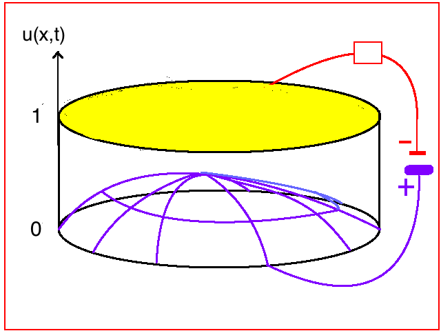 Figure 1: Two-membrane MEMS device
We consider a well-known model for micro-electromechanical systems (MEMS)
with variable dielectric permittivity, based on the following parabolic equation with singular nonlinearity:
where $\Omega$ is a smoothly bounded domain of $\mathbb{R}^2$ and
is a Hölder continuous function in .
In this mathematical model, the domain $\Omega$ represents the shape of the elastic plate in the horizontal direction, the solution $u=u(t,x)$ measures its vertical deflection,
while the function $f(x)$ is proportional to the constant voltage and characterizes the varying dielectric permittivity of the elastic plate.
We can write the permittivity profile $f$ as follows:
where $\lambda>0$ is the applied voltage, $\varepsilon_0>0$ is the permittivity of the vacuum and $\varepsilon_1(x)$ is the dielectric permittivity of the material.
As a key feature, in our model the permittivity of the elastic plate may be inhomogeneous,
and this can be used to trigger the properties of the device.
We refer to [1],[4],[5] and the references therein for the full details of the model derivation.
It is well known that problem (\ref{quenching problem}) admits a unique maximal classical solution $u$.
We denote its maximal existence time by $T=T_f\in (0,\infty]$. Moreover,
under some largeness assumption on $f$, it is known that the maximum of $u$ reaches the value $1$
at a finite time, so that $u$ ceases to exist in the classical sense. This is what we call touchdown in finite time $T_f<\infty$.
Actually, if we consider $f(x) = \lambda\dfrac{\varepsilon_0}{\varepsilon_1(x)}$,
it is well-known that there exists a positive $\lambda^\ast$, known as pull-in voltage, which depends on $\Omega$ and $\varepsilon_1(x)$, such that
$\bullet \quad $ If $\lambda<\lambda^\ast$, then $T_f=\infty$ and the global classical solution converges to the minimal positive steady state.
$\bullet \quad $ If $\lambda>\lambda^\ast$, then $T_f<\infty$, and then touchdown occurs in finite time.
In the actual design of a MEMS device there are several issues that must be considered.
Typically, one of the design goals is to achieve the maximum possible stable steady-state with relatively small applied voltage $\lambda$. Another consideration may be to increase the stable operating range of the device by increasing the pull-in voltage.
For other devices, such as micropumps and microvalves, where touchdown behavior is explicitly exploited,
it is of interest to be able to localize the touchdown points, or similarly, to be able to avoid touchdown in certain parts of the device.
Our approach to achieve this last goal is to consider a material with varying dielectric permittivity allowing us to localize the touchdown points by a suitable choice of the permittivity profile.
Results
We start by the definition of touchdown point.
A point $x = x_0$ is called a touchdown or quenching point if there exists a sequence ${(x_n , t_n )} \in \Omega\times (0, T)$ such that
The set of all such points is called the touchdown or quenching set, denoted by $\mathcal{T}=\mathcal{T}_f\subset\overline{\Omega}$.
We show in [2] that touchdown can actually be ruled out in subregions of $\Omega$
where $f$ is positive but suitably small, below a positive threshold.
Theorem 1:
Let $\Omega\subset \mathbb{R}^n$ a smooth bounded domain and $f$ a function satisfying
There exists $\gamma_0>0$ depending only on $\Omega,M,\mu,r$ such that:
(i) $\quad$ For any $x_0\in \Omega$, if $f(x_0) <\gamma_0 {\hskip 1pt} \text{dist}^3 (x_0,\partial\Omega)$, then $x_0$ is not a touchdown point.
(ii) $\quad $ For any $\omega\subset\subset \Omega$, if $\displaystyle\sup_{x\in \overline{\Omega}\setminus \omega} f(x) <
\gamma_0 {\hskip 1pt} \text{dist}^3(\omega,\partial\Omega)$, then the touchdown set
is contained in $\omega$.
Roughly speaking, the statement (i) in the above theorem allows one to rule out touchdown in an interior point by choosing a permittivity profile which is sufficiently small at that point, while statement (ii) allows to design devices producing touchdown inside any given subset of $\Omega$ by choosing a permittivity profile concentrated in that subset.
Numerical Simulation 1: no touchdown at the origin
In our first example, we consider a circular elastic plate of radius 1, that is $\Omega = B(0,1)\subset\mathbb{R}^2$.
It is well known that if the dielectric permittivity is constant, the unique touchdown point is the center of the disk.
As consequence of Theorem 1 (i), we can prevent touchdown to occur at the origin by choosing a permittivity profile $f$ such that $f(0)$ is sufficiently small.
Let’s assume that the applied voltage $\lambda$, together with the permittivity of the vacuum $\varepsilon_0$ and the permittivity of the material $\varepsilon_1$ are such that
In this case, we might cover the center of the disk with a material with higher permittivity so that the value of $\varepsilon_1(x)$ in $B(0,1/4)$ is (for example) twice its value in $\Omega\setminus B(0,1/4)$.
That is, we consider the following permittivity profile:
The following video represents the evolution of the elastic plate from the rest position to the pull-in instability.
For the numerical simulation we have applied an implicit Crank-Nicolson scheme in polar coordinates with number of meshpoint $N=100$ in the radial interval $[0,1]$.
Simulation 1: Evolution of the elastic plate until pull-in instability (touchdown). The solution reaches the value 1 in a circumference and then, touchdown is avoided at the center of the plate.
In the schematic video, we remove the upper plate of the MEMS device in order to see the final profile of the solution.
Numerical Simulation 2: touchdown near a prescribed circumference
Let us suppose now that we want our system to touch down in a circumference of radius near $0.7$.
This time we can use Theorem 1 (ii). We will choose a permittivity profile $f$ sufficiently concentrated near a circumference of radius $0.7$. Consider for example:
The following video represents the evolution of the elastic plate from the rest position to the pull-in instability.
In Figure 2 below, we plot the radial final touchdown profile.
For the numerical simulation we have applied an implicit Crank-Nicolson scheme in polar coordinates with number of meshpoint $N=100$ in the radial interval $[0,1]$.
Simulation 2: Evolution of the elastic plate until pull-in instability (touchdown). The solution reaches the value 1 in a circumference of radius near $0.7$.
In the schematic video, we remove the upper plate of the MEMS device in order to see the final profile of the solution.
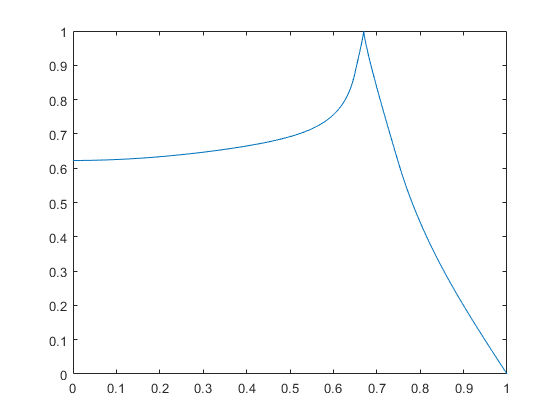
Figure 2: Plot of the radial touchdown profile. Observe that, as expected, touchdown occurs on a circumference of radius between $0.65$ and $0.75$.
Nontrivial touchdown sets
In view of Theorem 1,
it is a natural question whether such smallness conditions are actually necessary,
or whether touchdown could be shown to occur only at or near the maximum points of the permittivity profile $f$.
In this connection, using stability properties of the touchdown set,
in [2] we construct radial ‘‘M’‘-shaped profiles giving rise to
single-point touchdown at the origin.
Numerical simulation 3:
For this example, we have considered the following radial M-shaped profile in a disk of radius 1:
For this profile, the unique touchdown point is at the origin, far away from the maxima of $f$.
Therefore, if we want to prevent touchdown at the origin, we need to choose a permittivity profile $f$ such that $f(0)$ is small enough (below a certain thershold).
For the numerical simulation we have applied an implicit Crank-Nicolson scheme in polar coordinates with number of meshpoint $N=100$ in the radial interval $[0,1]$.
Simulation 3: Evolution of the elastic plate until pull-in instability (touchdown). Although we consider a ''M''-shaped permittivity profile, the solution touches down only at the origin, far away from the maximum of $f$.
In the schematic video, we remove the upper plate of the MEMS device in order to see the final profile of the solution.
Numerical simulation 4:
Another rather surprising example is the following radially increasing profile:
For this example, the unique touchdown point is the origin, which is actually the global minimum of $f$. In [2], we give a rigorous proof of the existence of this kind of behaviors. It is based on a stability result of the touchdown set combined with the fact that single-point touchdown occurs for constant permittivity profiles.
For the numerical simulation we have applied an implicit Crank-Nicolson scheme in polar coordinates with number of meshpoint $N=100$ in the radial interval $[0,1]$.
Simulation 4: Evolution of the elastic plate until pull-in instability (touchdown). Although the permittivity profile is radially increasing, the unique touchdown point is the origin, the minimum point of $f$.
In the schematic video, we remove the upper plate of the MEMS device in order to see the final profile of the solution.
Quantitative results in 1 dimension
Motivated by practical considerations of MEMS design, our aim in [3] is to further investigate the
touchdown localization problem
and to show that in one space dimension, where analytic computations can be made more precise,
one can obtain quite quantitative conditions.
Namely, we look for a lower estimate of the ratio $\rho$ between $f$ and its maximum,
below which no touchdown occurs on a subregion of $\Omega$.
Rather surprisingly, it turns out that, under suitable assumptions on $f$,
our methods yield values of
the threshold-ratio $\rho$ which are not ‘‘small’’ but can actually be up to the order
which could hence be quite appropriate for robust practical use.
In order to give good estimates of the ratio $\rho$, we shall consider two typical situations, which roughly correspond to a one-bump or a two-bump shape for the profile $f$.
The touchdown is ruled out in a subinterval respectively located between a bump and
an endpoint of $\Omega$, or between two bumps.
The idea behind this is that the plate can be covered with two dielectric materials,
one with a high permittivity and the other with a lower permittivity. We then seek for a ratio between the two permittivities, allowing to rule out touchdown in the low permittivity region.
Reduction to a finite-dimensional optimization problem
As a consequence of our method, the threshold-ratio $\rho$ is rigorously obtained as the solution of a suitable finite-dimensional optimization problem, with either three or four parameters.
An advantage of our results is that they apply to large classes of configurations, so that detailed numerics need not be carried out to localize the touchdown set for particular cases.
For the precise statements of the results, as well as for a detailed study of the optimization problem and numerical estimates of the threshold ratio, we refer the lector to [3].
The Matlab codes to compute numerical estimates of the solution of the optimization problem are availabe at the beginig of the page.
Here we give two concrete examples in order to illustrate
the results.
The threshold ratio is obtained by a simple numerical procedure applied to the finite-dimensional optimization problem.
The following two figures represent some typical permittivity profiles $f(x)$ and the localization of the corresponding touchdown sets
in the one-bump and two-bump cases respectively.
The touchdown sets are localized in a neighborhood of the bumps, represented by the fat lines.
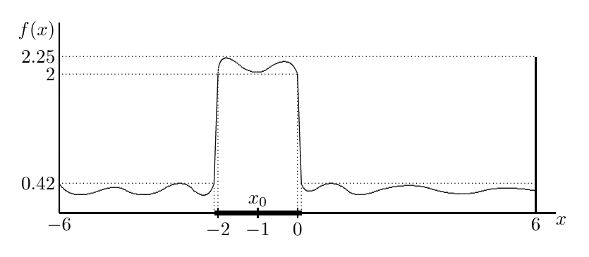 Figure 3: An illustration of the localization of thouchdown set for a one-bump permittivity profile.
Here, the figure represents the permittivity profile $f$ and not the profile of the solution.
Figure 3: An illustration of the localization of thouchdown set for a one-bump permittivity profile.
Here, the figure represents the permittivity profile $f$ and not the profile of the solution.
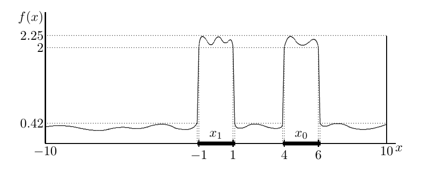 Figure 4: An illustration of the localization of thouchdown set for a two-bump permittivity profile.
Here, the figure represents the permittivity profile $f$ and not the profile of the solution.
Figure 4: An illustration of the localization of thouchdown set for a two-bump permittivity profile.
Here, the figure represents the permittivity profile $f$ and not the profile of the solution.
Numerical simulation 5:
We give an example of a one-bump permittivity profile, similar to the one in Figure 3.
Although our result applies to a large class of profiles, here we consider, for computational simplicity, the following bang-bang profile:
The following video represents the evolution of a 1-dimensional membrane
with a one-bump permittivity profile $f$.
For the numerical simulation we have applied an implicit Crank-Nicolson scheme with number of meshpoint $N=1000$ in the interval $[-6,6]$.
Simulation 5: Evolution of the elastic 1-dimensional membrane until pull-in instability (touchdown). We see that touchdown is localized in the region where $f$ is big (see Figure 3).
Numerical simulation 6:
We give an example of a two-bump permittivity profile, similar to the one in Figure 4.
Although our result applies to a large class of profiles, here we consider, for computational simplicity,
the following bang-bang profile:
The following video represents the evolution of a 1-dimensional membrane
with a two-bump permittivity profile $f$.
For the numerical simulation we have applied an implicit Crank-Nicolson scheme with number of meshpoint $N=1000$ in the interval $[-10,10]$.
Simulation 6: Evolution of the elastic 1-dimensional membrane until pull-in instability (touchdown). We see that touchdown is localized in the region where $f$ is big (see Figure 4).
References
[1] P. Esposito, N. Ghoussoub, Y. Guo, Mathematical analysis of partial differential equations modeling electrostatic MEMS. Courant Lecture Notes in Mathematics, 20. Courant Institute of Mathematical Sciences, New York; American Mathematical Society, Providence, RI, 2010. xiv+318 pp.
[2] C. Esteve, Ph. Souplet, No touchdown at points of small permittivity and nontrivial touchdown sets for the MEMS problem. Advances in Differential Equations, Vol 24, Number 7-8(2019), 465-500.
[3] C. Esteve, Ph. Souplet, Quantitative touchdown localization for the MEMS problem with variable dielectric permittivity. Nonlinearity} 31 4883 (2018).
[4] Ph. Laurençot, Ch. Walker, Some singular equations modeling MEMS. Bull. Amer. Math. Soc. 54 (2017), 437-479.
[5] J.A. Pelesko, D.H. Bernstein, Modeling MEMS and NEMS, Chapman Hall and CRC Press, 2002.