Introduction
GPS enabled devices, such as smart phones, have gained large popularity in the last few years. It allows people to record their outdoor activities through GPS trajectories, which enables researchers to infer further knowledge about the moving behavior of mobile users [8]. An important topic in analyzing GPS data is the identification of significant or interesting places visited by users [1] because if we extract them, we can know each user well and this will allow us to have a better prediction on the user’s next location.
Generally, a prediction problem involves using past observations to predict or forecast one or more possible future observations. The goal is to guess about what might happen in the future. Knowing the future can impact our decisions today so we have a great interest in predicting it.
In this project we tried first working on finding an algorithm that can help us define the points of interest of the users we have in the dataset. For that we implement an algorithm that can identify the users stop points.
Next step was predicting the next location of the users to do that we used different approaches (Markov chains, Random forest and Recurrent neural network).
KEYWORDS: GPS Trajectory; Clustering algorithm; Points of interests (POI); Prediction; Markov chain; Random Forest; DBSCAN; HDBSCAN.
Motivation
With the popularity of smartphones and other equipment that can be used to record locations via the Global Navigation Satellite System (GNSS) [8], capturing and recording trajectory data based on such equipment becomes more convenient. The smartphone for exemple combines different sophisticated features. It allows users to keep pictures, memories, personal info, health [9,10] etc. And with each use to some application we can get the user GPS coordinates at a period of time [11].
So why don’t we use this data to better understand the users? If we get to know the next step of each individual we can for example suggest some near restaurants, shops and places they used to go to, or notify them if someone they know is close to where they are.
It could be also beneficial for the police department [12], it can help them identify criminals’ places or finding missing people and more likely it can also help people with Alzheimer’s, by notifying their relatives about their places.
Problem statement
Mobility is part of human’s daily life. We move from one place to another for different reasons. For example we go to a certain place to work and to another place to meet people.
Mobility patterns of users have been studied intensively. The ubiquity of mobile phones with their embedded sensors and available applications opened new possibilities both for academia and industry to study human mobility patterns [2,3].
In this project the main objective is to extract the useful data from different users trajectories in order to predict their next locations afterwards.
Presentation of our data
In this project we are working on a time series dataset (see Fig. 1) that contains 288 user GPS coordinates of three month (March, April, May). These users lives in Spain.
The data was collected whenever the users are connected to their accounts.
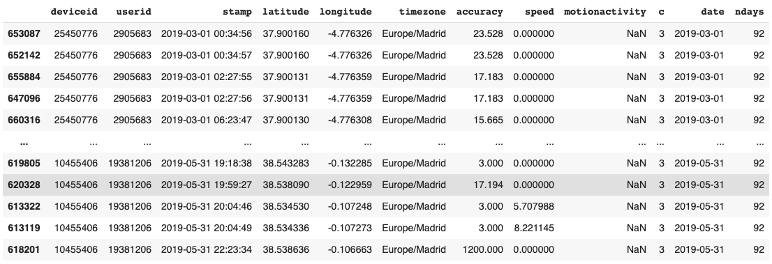 Figure 1. Time series database of GPS coordinates.
We can see in Figure 2 the representation of 10\% of the users on the map. As we can notice the users are so active inside and outside of Spain. In Figure 3 we see the GPS representation of a user on the map.
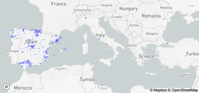 Figure 2. Represantation of 10\% of the users population we have on the map.
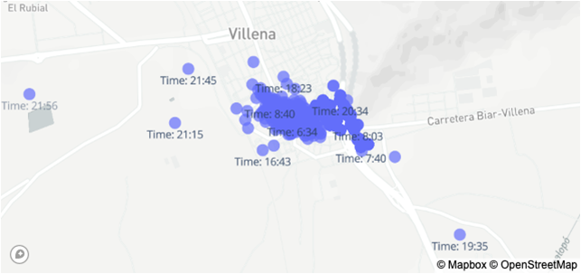 Figure 3. Representation of one user GPS coordinates on the map.
Methodology
The first objective is to extract the points of interest (POIs) which represent the locations that the individual visit frequently (Home, Place of work, gym \dots, etc), of the different users we have in the dataset after grouping it by users so that it would be easy to analyse them separately.
Working on a real world data means the existence of noise the first two clustering algorithms (K-means and GMM) as we can see in Figures 4 y 5 they weren’t capable of eliminating the noise in our data, because in these algorithms each point must belong to one cluster which is not convenient for our data, not all the points are part of a location some points shows us only the trajectory that the user did to get to the desired place so we can say that these two approaches are not able to differentiate between a stop point and a trajectory.
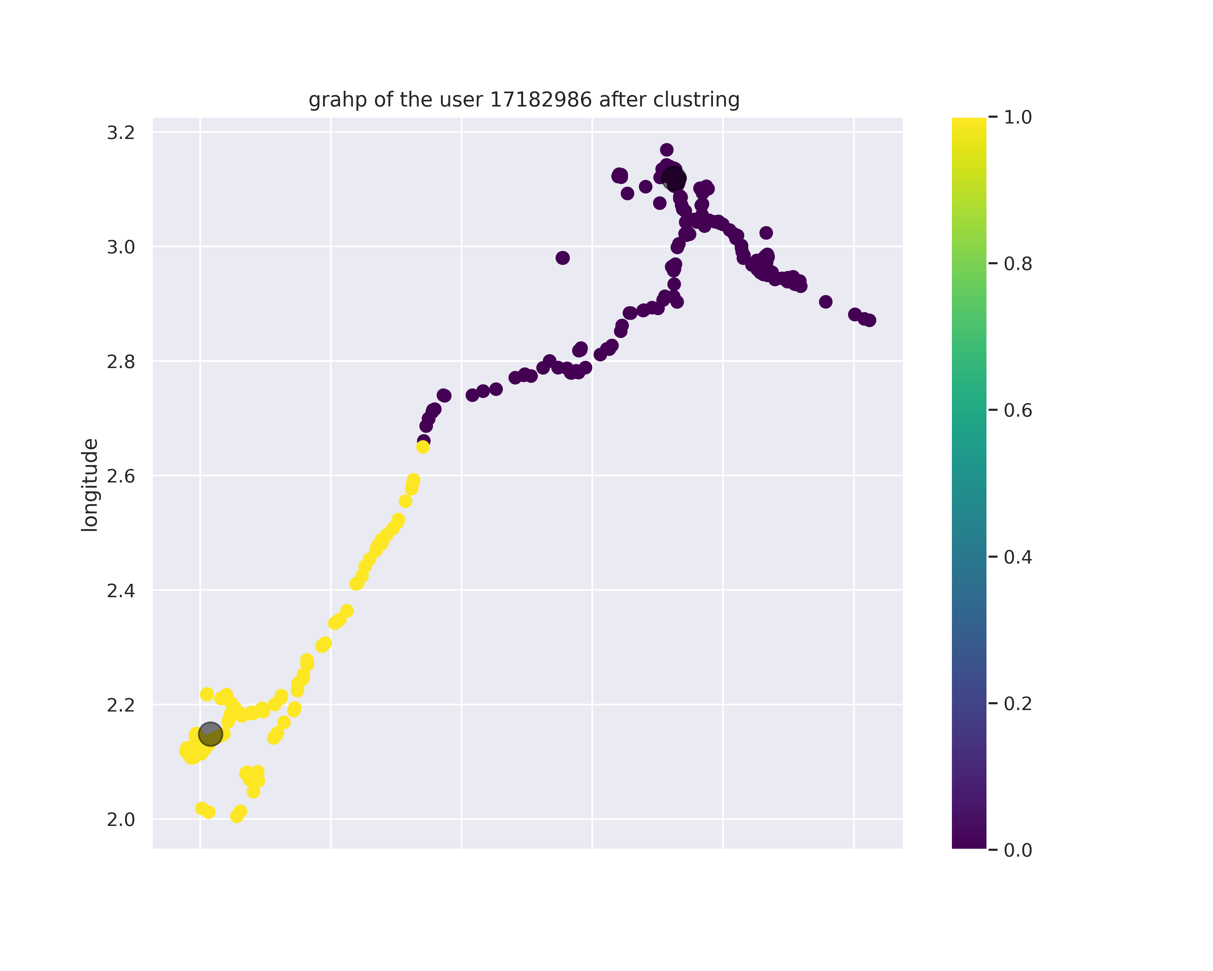 Figure 4. Graphic representation of a user GPS coordinations after k-means clustering.
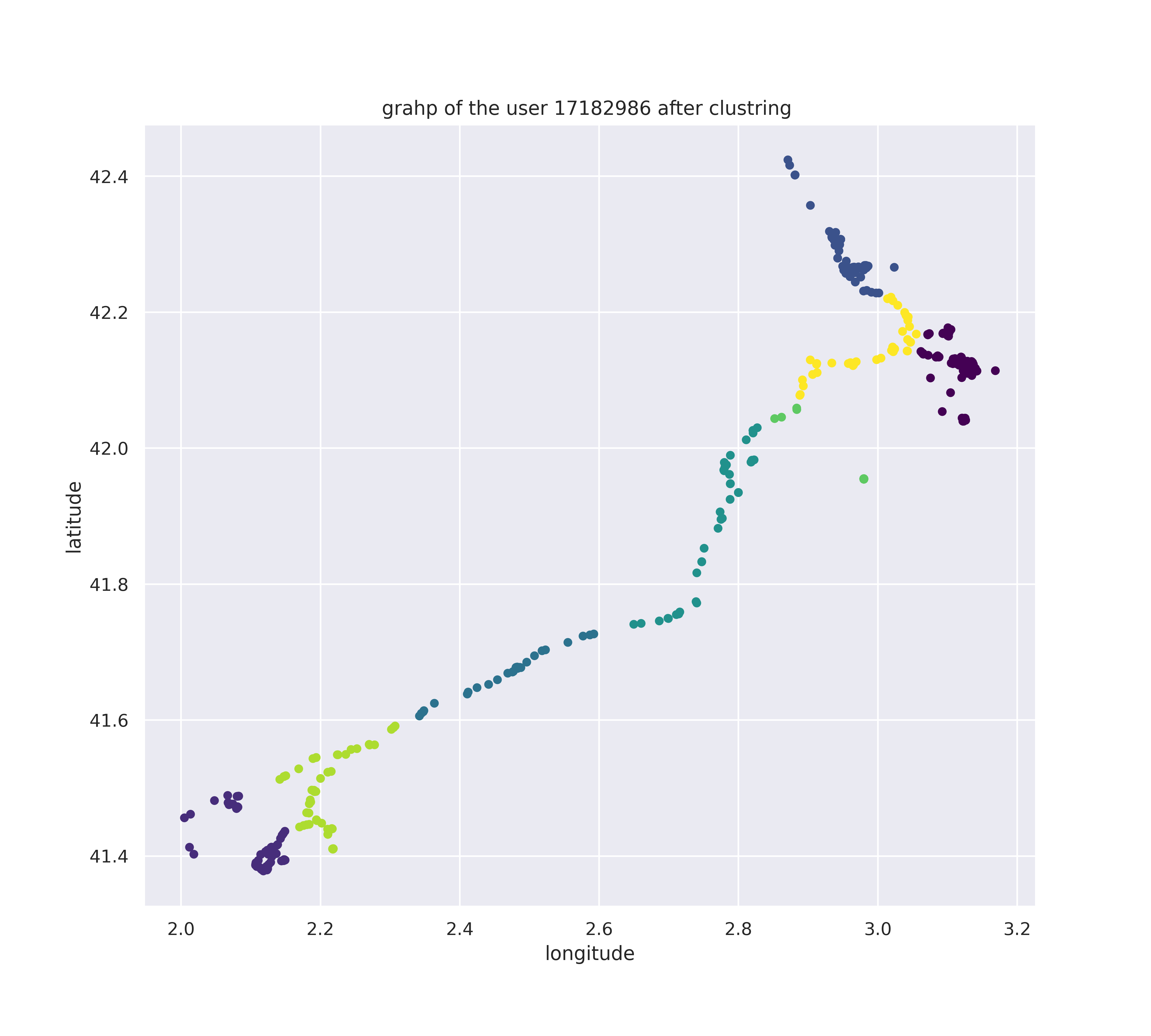 Figure 5. Graphic representation of a user GPS coordinations after GMM clustering.
So we had to look for other approaches that can eliminate the noise. The first algorithm we tried was DBSCAN [6], but it wasn’t easy for us to estimate the best parameters, especially that each user has it’s proper trajectory and also the density of the points wasn’t unified for the same user, some group of points are so close to each other then others.
For that the next algorithm we used was HDBSCAN [5] because in this algorithm the threshold is not fixed so it’s capable of identifying clusters of different densities. This algorithm gives us some good results but after implementing the clusters on the map we can see that for some users the clusters didn’t include just the meaningful points but also some of the noise (the trajectory of the user) as we can see in Figure 4.
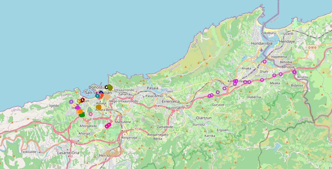
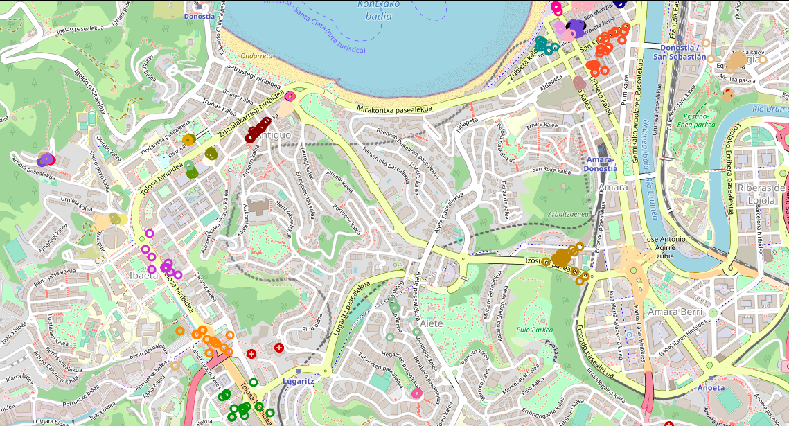 Figure 6. Implementation of a user clusters on the map after removing the noise with HDBSCAN
For that we needed to implement an algorithm that can identify the users stop points, which tells us where and when a user has stopped (stayed). It consists of a timestamp, a user identifier as well as longitude and latitude coordinates. It also has two additional variables: t_start and t_end indicating the start-time and end-time of the stop (see Figure 5).
The stop location extraction algorithm [7] has two parameters which are dependent on the application:
$\bullet \quad $ Roaming distance: defines how far a user is allowed to roam to still be considered part of the stop location (dashed orange line
$\bullet \quad $ Stay duration: specifies the minimum amount of time a user has to stay within the roaming distance for his position to be considered as being part of a particular stop location.
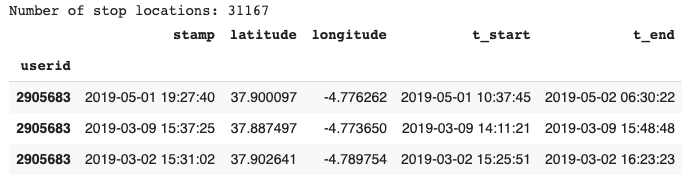 Figure 7. Output of the stop algorithm.
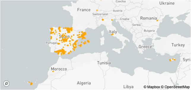 Figure 8. Representation of the stop points of the users on the map.
The next step is to aggregates stop locations in close proximity of each other to know where and how often a user has stopped at a destination. The destination consists of a timestamp, a user identifier as well as latitude and longitude coordinates. In addition, the visitation count denotes the number of stops at a particular destination and cluster_assignment identifies the destination itself.
What we are actually interested in is the destination where a user has stopped and not necessarily the exact GPS position recorded. For instance, the group of stop locations surrounding a building should be regarded as one destination. In other words, we need to cluster or aggregate the stop locations into destinations (see Figure 7).
To aggregate the stop locations into destinations we use Scipy’s hierarchical clustering functions (see Figure 8). For our application there are two important parameters: \emph{The linkage parameter} defines how the clusters are formed. \emph{The distance parameter} specifies within what spatial distance stop locations are to be considered of the same cluster.
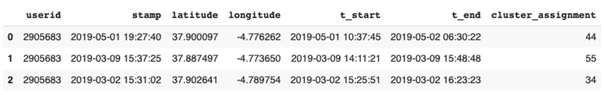 Figure 9. Output of destination algorithm
To get medoid for each destination, now that we have assigned each stop location to a destination, we want to have only one point representing each destination.
To have one representative point per cluster, we calculate the medoid of the stop locations within each destination. We also calculate the number of stop locations at each destination, which is useful for ranking destinations based on visitation counts.
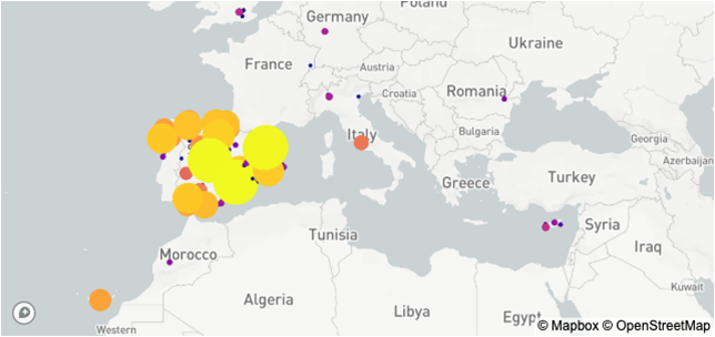
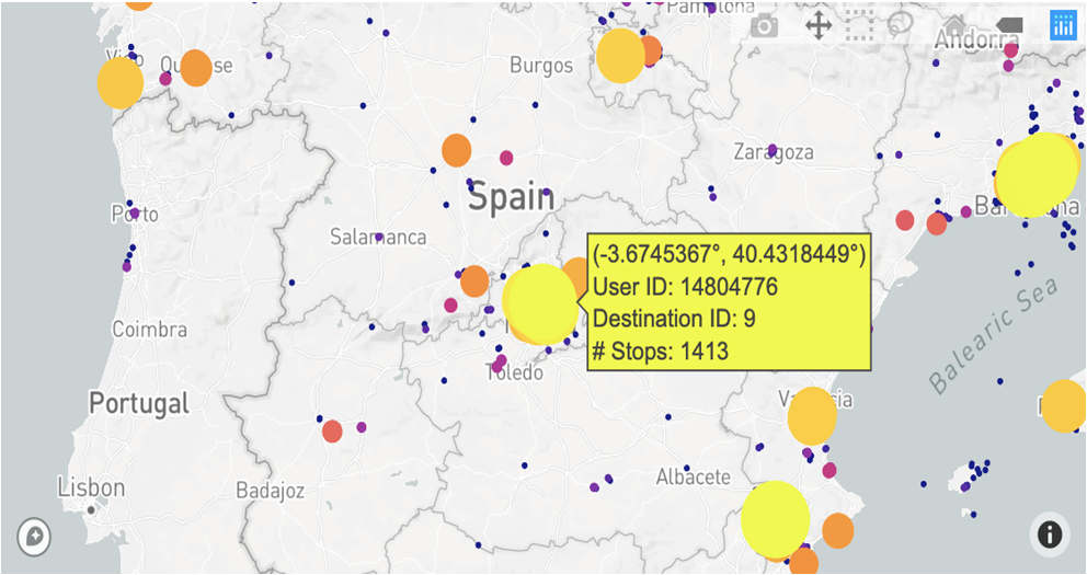 Figure 10. Representation of the users destinations on the map.
Next step is to predict n-next steps to do that we use two different approaches the markov chains and random forest. But before that we need to split our data into two parts train which we give 90\% of our data and the rest(10\%) to the test.
After running the hidden markov chains model on our data we get to predict the next clusters of each user. We are predicting the clusters because each cluster represent a POI.
After training our model we calculate the accuracy of it for each user and to get the general accuracy score we get the mean score and it was 49\%. that means that our model is not that good at predicting the next location.
So the next approach we used is random forest which is a supervised learning algorithm that can be used for class classification or regression (prediction).
The accuracy of Random forest model is 94\% which shows that the model is doing well at predicting the users next locations.
References
[1] S. Gambs and M.O. Killijian, Next Place Prediction using Mobility Markov Chains, MPM’12, April 10, 2012, Bern, Switzerland.
[2] Z. Fu, Z. Tian, Y. Xu and C. Qiao, A Two-Step Clustering Approach to Extract Locations from Indi- vidual GPS Trajectory Data, ISPRS Int. J. Geo-Inf. Vol. 5, 166, 1–17, 2016. doi:10.3390/ijgi5100166
[3] N. Palmius and A. Tsanas and K. E. A. Saunders and A. C. Bilderbeck and J. R. Geddes and G. M. Goodwin and M. De Vos, Detecting Bipolar Depression From Geographic Location Data, IEEE Trans Biomed Eng., Vol. 64, No. 8, 1761–1771, 2017. doi: 10.1109/TBME.2016 2611862
[4] J. Busk and M. Faurholt-Jepsen and M. Frost and J. E. Bardram and L. Vedel Kessing and O. Winther, Forecasting Mood in Bipolar Disorder From Smartphone Self-assessments: Hierarchical Bayesian Approach, JMIR Mhealth Uhealth, Vol. 8, No. 4, 1–14, 2020
[5] P. Widhalm and P. Nitsche and N. Brandie, Transport mode detection with realistic Smartphone sensor data. In Proceedings of the International Conference on Pattern Recognition, Tsukuba, Japan, 11–15 November 2015; IEEE: Piscataway, NJ, USA, 2012; 573–576.
[6] A. Bogomolov and B. Lepri and J. Staiano and N. Oliver and F. Pianesi and A. Pentland, Once Upon a Crime: Towards Crime Prediction from Demographics and Mobile Data. In Proceedings of the 16th International Conference on Multimodal Interaction, Istanbul, Turkey, 12–16 November 2014; ACM: New York, NY, USA, 2014; 427–434.
[7] V. Bogorny, C. Renso, A.R. de Aquino, F. de Lucca Siqueira and L.O. Alvares, Constant–A Con- ceptual Data Model for Semantic Trajectories of Moving Objects, Trans. GIS Vol. 18, 66–88, 2014.
[8] L. Xiang, M. Gao and T. Wu, Extracting Stops from Noisy Trajectories: A Sequence Oriented Clustering Approach, ISPRS Int. J. Geo-Inf. Vol. 5, 29, 1–18, 2016. doi:10.3390/ijgi5030029
[9] Ester M., Kriegel H.P., Sander J. and Xu X. A density-based algorithm for discovering clusters in large spatial databases with noise. KDD-96 Proceedings, 226–231, 1996
[10] Campello R.J.G.B., Moulavi D., Sander J. Density-Based Clustering Based on Hierarchical Density Estimates. In: Pei J., Tseng V.S., Cao L., Motoda H., Xu G. (eds) Advances in Knowledge Discovery and Data Mining. PAKDD 2013. Lecture Notes in Computer Science, Vol. 7819. Springer, Berlin, Heidelberg, 2013.
[11] R. Hariharan and K. Toyama. Project Lachesis: Parsing and Modeling Location Histories. KDD- 96 Proceedings, In: Egenhofer M.J., Freksa C., Miller H.J. (eds) Geographic Information Science. GIScience 2004. Lecture Notes in Computer Science, Springer, Berlin, Heidelberg, Vol. 3234, 106– 124, 2004
[12] Camacho-Lara, S. Current and Future GNSS and Their Augmentation Systems In: Handbook of Satellite Applications; Springer Science and Business Media LLC: Berlin, Germany, 2013, pp. 617?654.