Opening the black box of Deep Learning
Deep Learning is one of the three main paradigms of Machine Learning, and roughly consists on extracting patterns from data using neural networks.
Its impact in modern technologies is huge. However, there is not a clear high-level description of what these algorithms are actually doing.
In this sense, Deep Learning models are sometimes referred to as “black box” models”; that is, we can characterize the models by its inputs and outputs, but with any knowledge of its internal workings.
The aim is then to open the black box of Deep Learning, and try to gain an intuition of what are these models doing.
One of the most succesful mathematical theories in recent years has been connecting Deep Learning with Dynamical Systems.
The aim of this post is to introduce to some of those exciting ideas.
Data and classification
Supervised Learning
Deep Learning essentially wants to solve the problem of Supervised Learning. That is, we want to learn a function that maps an input to an output, based on examples of input-output pairs.
A classical Deep Learning problem would be the following: we have some pictures of cats and dogs, and want to make an algorithm that learns when the input image shows a dog and when it shows a cat. Note that we could give the algorithm pictures that it has not previously seen, and the algorithm should label the pictures correctly.
A formal description of our problem is the following.
Consider a dataset $\mathcal{D}$ consisting on $S$ distinct points ${x_i}_{i=1}^{S}$, each of them with a corresponding value $y_i$ such that
we expect that the labels $y_i$ are a function of $x$, such that
where $\epsilon _i$ is included so as to consider, in principle, noisy data.
The aim of supervised learning is to recover the function $\mathcal{F}(\cdot)$ such that not only fits well in the database $\mathcal{D}$ but also generalises to previously unseen data.
That is, it is inferred the existence of
where
being $\mathcal{F} (\cdot)$ the desired previous application, and $\mathcal{D} \subset \tilde{\mathcal{D}}$.
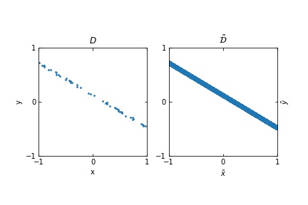 Figure 1. *The figure in the left represents a finite set of points in $(x,y)$, where $x$ represents the input and $y$ the output. The figure on the right is the expected distribution from which we are sampling the input-output examples. The whole distribution can be understood by $\tilde{\mathcal{D}}$.*
A well-known dataset in which to use Deep Learning algorithm is the CIFAR-10 dataset.
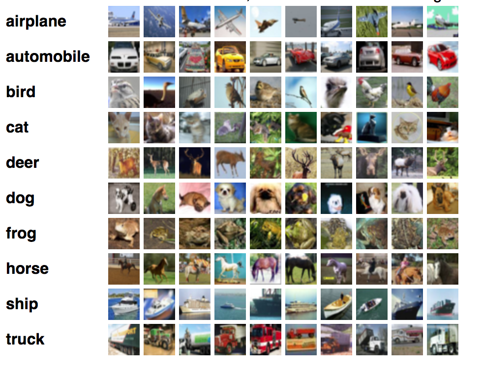 Figure 2. Scheme of the CIFAR-10 dataset.
In this case, the input images consist on a value in $[0,1]$ for each pixel and Red / Green / Blue color. Since the resolution is $32 \times 32$ pixels, the input space would be $[0,1]^d$ with $d=32 \times 32 \times 3 = 3072$. Each image has a correspondent label (airplane, automobile, …).
The dataset is then given by $ { x_j, y_j = f^{\star(x_j)} } $ where the inputs $ x_j \in [0,1]^{3072} $, and the labelling function acts as $f^* : [0,1]^{3072} \to { \text{airplane, automobile, … } }$.
We want that $ f^*( \text{each image} ) = \text{correct label of that image} $.
Note that the function $ f^* $ we are talking about is not the same as the function $\mathcal{F}$ that we used when defining the notion of dataset. This is because the function $ f^* $ is the application that connects the images with their given labels, whereas the function $\mathcal{F}$ is the function that connects any feasible input image with its true label. We have access to $f^*$, but not $\mathcal{F}$.
Noisy vs. noisless data
What are the true labels of a dataset? We have no a priori idea. What is the mathematical definition of “pictures of airplanes”? Our best guess is to learn the definition by seing examples.
However, those examples may be mistakenly labelled, since the datasets are in general noisy. What does a noisy dataset mean?
-
We refer to noisy data when the samples in our dataset $\tilde{\mathcal{D}}$ actually comes from a random vector $(\mathbf{x}, \mathbf{y})$ with a non-deterministic joint distribution, such that it is not possible to find a function $\mathcal{F}$ such that $\mathcal{F}(\mathbf{x}) = \mathbf{y}$.
The aim of supervised learning, in this case, would be to find a function such that
$\mathcal{F}(\mathbf{x}) \approx \mathbf{y}$. For example, $\mathcal{F}(\tilde{x}_i) = \tilde{y}_i$ for almost every sample $i$.
-
In the case of noisless data (which does not happen in most practical situations, but it makes things far simpler) then it is possible to find a function $\mathcal{F}$ such that $\mathcal{F}(\tilde{x}_i) = \tilde{y}_i \; \forall i$, or equivalently $\mathcal{F}(\mathbf{x}) = \mathbf{y}$.
Note that, given that the probability of a collision (of having two different data-points such that $x_i = x_j$ for $i \neq j$) is practically $0$, it is in principle possible to find a function $\mathcal{F}$ such that $\mathcal{F}(x_i)=y_i$ for all of our samples i, even in the noisy case (for example, we may use interpolation).
However, the aim of supervised learning is to be able to generalise well to previously unseen data, $\tilde{\mathcal{D}}$, and so interpolation is not effective, and may not be well-defined, since the same input $x_i$ can be labelled differently, due to noise.
Representation of the optimal function $\mathcal{F}$ as the number of samples increases, in the case of noisy data. Note that the function “stabilizes” at a certain point, and thus it is expected to behave properly in the limit of infinitely many samples.
 Representation of the optimal function $\mathcal{F}$ as the number of samples increases, in the case of noisless data. In this case the function could have been obtained by interpolation, and would stabilize fast.
Binary classification
In most cases, the data points $x_i$ are in $\mathbb{R}^{n}$. In general, we may restrict to a subspace of feasible images $X \in \mathbb{R}^{n}$.
So as to ease the training of the models, the inputs are usually normalized, and it is considered $X = [-1,+1]^{n}$, with $n$ the input dimension.
There are different supervised learning problems depending on the space $Y$ of the labels.
If $Y$ is discrete, such that $Y = { 0, … , L-1}$, then we are dealing with the problem of classification. In the case of CIFAR-10 we have $10$ classes, and so $L=10$.
If $L=2$, then it is a binary classification problem, such as in the case of classifying images of cats and dogs (in this case, dog may be represented by “0” and cat by “1”).
In the particular setting of binary classification, the aim is to find a function $\mathcal{F} (x)$ such that it returns $0$ whenever the corresponding data point $x$ is of class $0$, and $1$ conversely.
Data, subspaces and manifolds
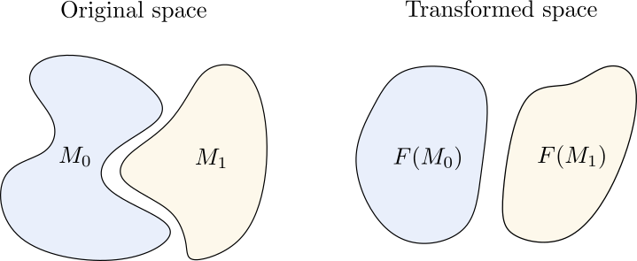
Consider $M^0$ the subset of $X$ such that $F( \tilde{x} _i) =0$ for all the points $\tilde{x}_i$ in $M^0$. And consider $M^1$ such that $\, F(\tilde{x}_i)=1$ for all the points in $M^1$.
It is useful to consider $d(M^0 , M^1) > \delta$. That is, we want the subspace of images of cats and the subspace of images of dogs to have a nonzero distance in the input space. This makes sense physically, since we do not expect the pictures of dogs and cats to overlap.
An interesting hypothesis is to consider that $M^0$ and $M^1$ are indeed manifolds in a low-dimensional space. This is called the manifold hypothesis.
That is, out of the whole input space of all possible images, only a low-dimensional subspace of those would correspond to the images of cats, and one could go from one picture of a cat to any other picture of a cat by a path in which all the point are also pictures of cats. This has been widely hypothesized in many datasets, and there are some experimental results in that direction [9].
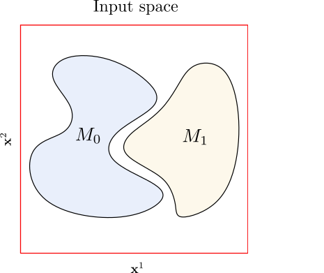 Example of the input space in a binary classification setting. The axis $\mathbf{x}^1$ and $\mathbf{x}^2$ represent the components of the vectors $x$ the input space (we are considering $[0,1]^2$). The points in the subspace $M_0$ are labelled as $0$, and the points in $M_1$ as $1$. The points that are not in $M_0$ or $M_1$ do not have a well-defined label
Deep Learning
Now that we have some inuition about the data, it’s time to focus on how to approximate the functions $f$ that would fit that data.
When doing supervised learning, we need three basic ingredients:
- An hypothesis space, $\mathcal{H}$, consisting on a set of trial functions. All the functions in the hypothesis space can be determined by some parameters $\theta$. That is, all the functions $f \in \mathcal{H}$ are given by $f ( \cdot ; \theta )$. We therefore want to find the best parameters $\theta ^*$.
- A loss function, that tells us how close we are from our desired function.
- An optimization algorithm, that allows us to update our parameters at each step.
Our algorithm consists on initializing the process by choosing a function $f( \cdot , \theta) \in \mathcal{H}$. In Deep Learning, this is done by randomly choosing some parameters $\theta _0$, and initializing the function as $f( \cdot ; \theta_0)$.
In Deep Learning, the loss function is given by the empirical risk. That is, we choose a subset of the dataset,
and compute the loss as
, where
could be simply given by
.
The optimization algorithms used in Deep Learning are mainly based in Gradient Descent, such as
Where the subindex denotes the parameters at each iteration.
We expect our algorithm to converge; that is, we want that, as $k \to \infty$, we would have $\theta_{k}$ close to $\theta^*$, where the notion of “closeness” is given by the chosen loss function.
Paradigms of Deep Learning
There are many questions about Deep Learning that are not yet solved. Three of that paradigms, that woud be convenient to treat mathematically, are:
- Optimization: How to go from the initial function, $F_0$, to a better function $\tilde{F}$? This has to do with our optimization algorithm, but also depends on how do we choose the initialization, $F_0$.
- Approximation: Is the ideal solution $ F^* $ in our hypothesis space $\mathcal{H}$? Is $\mathcal{H}$ at least dense in the space of feasible ideal solutions $ F^* $ ? This is done by characterizing the function spaces $\mathcal{H}$.
- Generalization: How does our function $\tilde{F}$ generalise to previously unseen data? This is done by studying the stochastic properties of the whole distribution, given by the generalised dataset.
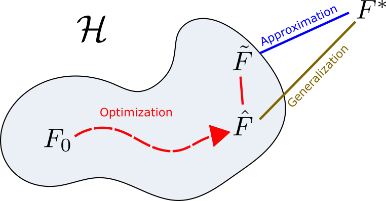 Diagram of the three main paradigms of Deep Learning. The function $F_0$ is the initial one, $\tilde{F}$ is the final solution as updated by the optimization algorithm, $\hat{F}$ is the closest function in $\mathcal{H}$ to $F^*$, and $F^*$ is the best ideal solution.
The problem of approximation is somehow resolved by the so-called Universal Approximation Theorems (look, for example, at the results by Cybenko [11]). This results state that the functions generated by Neural Networks are dense in the space of continuous functions. However, in principle it is not clear what do we gain by increasing the number of layers (using deeper Neural Networks), that seem to give better results in practuce.
Regarding optimization, altough algorithms based in Gradient Descent are widely used, it is not clear whether the solution gets stucked in local minima, if convergence is guaranteed, how to initialize the functions…
When dealing with generalization, everything gets more complicated, because we have to derive some properties of the generalised dataset, from which we do not have access. It is probably the less understood of those three paradigms.
Indeed, those three paradigms are very connected. For example, if the problem of optimization is completely solved, we would know that our final solution given by the algorithm, $\tilde{F}$, would be the best possible solution in the hypothesis space, $\hat{F}$; and if approximation is solved, we would also end up getting the ideal solution $F^*$.
One of the main problems regarding those questions is that the hypothesis space $\mathcal{H}$ is generated by a Neural Network, and so it is quite difficult to characterize mathematically. That is, we do not know much about the shape of $\mathcal{H}$ (although the Universal Approximation Theorems give valuable insight here), nor how to “move” in the space $\mathcal{H}$ by tuning $\theta$.
Let’s take a look at how the hypothesis spaces look like.
Hypothesis spaces
In classical settings, an hypothesis space is often proposed as
where $\theta = { a_i }_{i=1}^{m}$ are the coefficients, ${ \psi _i}$ are the proposed functions (for example, they would be monomials if we are doing polynomial regression).
The function $\mathcal{F}$ correspondent to the dataset $\mathcal{D}$ is then defined as
where $d$ is a distance defined by a loss function, and $\phi$ is a function that transforms $f(x_i; \theta)$ such that we can compare it with $y_i$. For example, if we want to do binary classification, we would use $\phi$ as a function that divides the space into two hiperplanes, and assigns $0$ to one of the parts of the divided space, and $1$ to the other.
This means that it is the function in the hypothesis space that minimizes the distance with the target function, which connects the datapoints $x_i$ with their correspondent labels $y_i$.
When using Deep Neural Networks, the hypothesis space $\mathcal{H}$ is generated by the composition of simple functions $f$ such that
where $\theta = { \theta_k }_{k=1}^{L}$ are the training weights of the network and $L$ the number of hidden layers.
Multilayer perceptrons
In the case of the so-called multilayer perceptrons, the functions $f^k_{\theta_k}$ are constructed as
being $A^k$ a matrix, $b^k$ a vector, $\theta _k =
{A^k , b^k}$ and $\sigma \in C^{0,1}(\mathbb{R})$ a fixed nondecreasing function, called the activation function.
Since we restrict to the case in which the number of neurons is constant through the layers, we have that $A^k \in \mathbb{R}^{d \times d}$ and $b^k \in \mathbb{R}^d$.
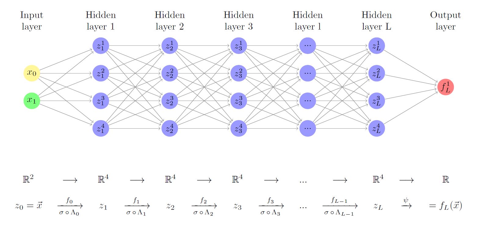 Diagram of a multilayer perceptron, also called fully-connected neural network. However, this graph representation seems a bit difficult to treat, so we use an algebraic representation instead
That is, shematically, one has that $\mathcal{H} = { F : F(x) = F_T \circ F_{T-1} \circ … \circ F_0 (x) }$, the hypothesis space is generated by the discrete composition of functions.
It can be seen that the complexity of the hypothesis spaces in Deep Learning is generated by the composition of functions. Unfortunately, the tools regarding the understanding of the discrete composition of functions are quite limited.
Moreover, considering $b^k=0$, we have that $F(x) = \sigma \circ A_T \circ \sigma \circ A_{T-1} \circ … \circ \sigma A_0 \circ x$. The gradient would then go as $\nabla_\theta F \sim A_T \cdot A_{T-1} \cdot … \cdot A_0 \sim k^L$. For $L$ large, the gradients would become very large or very small, and so training would not be feasible by gradient descent.
This is one of the reasons for introduction the Residual Neural Networks.
Residual Neural Networks
In the simple case of a Residual Neural Network (often referred to as ResNets) the functions $f_{\theta_k}^{k} (\cdot)$ are constructed as
where $\mathbb{I}$ is the identity function. The parameters $\sigma$, $A^k$ and $b^k$ are equivalent to those of the multilayer perceptrons.
We will see that it is sometimes convenient to numerically add a parameter $h$ to the residual block, such that
being $h \in \mathbb{R}$ a scalar.
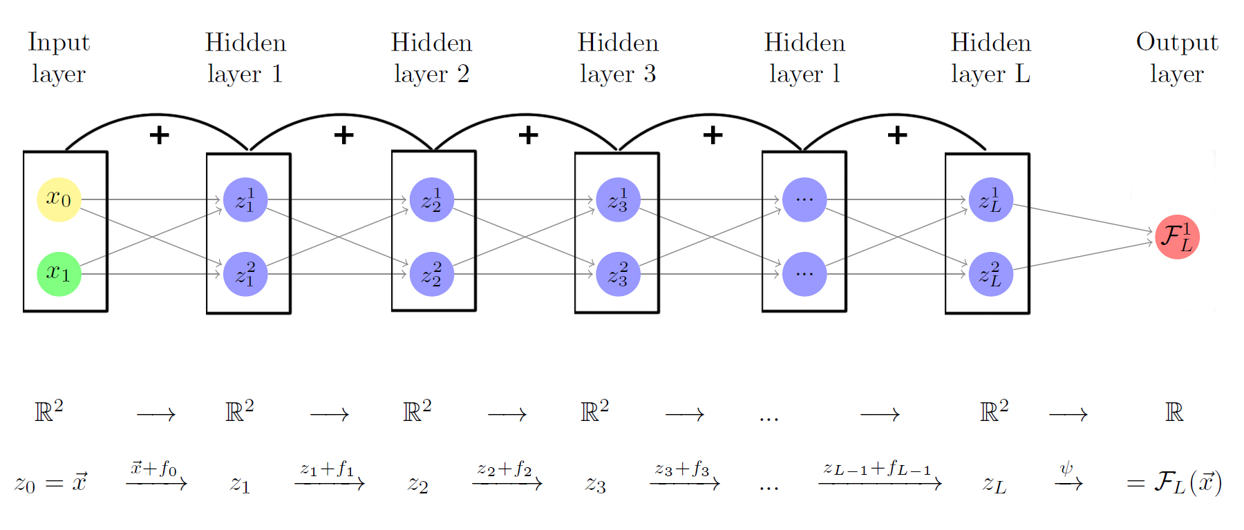 Diagram of a ResNet, in a graph manner. Again, an algebraic representation is preferred.
Visualizing Perceptrons
The Neural Networks then represent the compositions of functions $f$, which consist on an affine transformation plus a nonlinearity.
If we use the activation function $\sigma ( \cdot ) = tanh (\cdot)$, then each function $f$ (and so each layer of the Neural Network) is first rotating and translating the original space, and then “squeezing” it.
 Example of the transformation of a regular grid by a perceptron.
Binary classification with Neural Networks
When dealing with data classification, it is very useful to just assign a color / shape to every label, and so be able to visualize data in a lower-dimensional plot.
The aim of classification is to associate different classes to different regions of the initial space,
When using Neural Networks, the initial space $X$ is propagated by the Neural Network as $F = f ^L \circ f^{L-1} \circ … \circ f^1 (X)$.
Then the function $\phi$ would divide the space by an hyperplane, associate $0$ to one region and $1$ to the other.
So, while it may be difficult to classificate the datapoints in the initial space $X$, the Neural Networks should make things simpler and just propagate the data so as to make it linearly separable (and we would see this in real action!).
Our aim is therefore to transform the initial space $X$ in such a way that $M^0$ and $M^1$ are linearly separable. That is,
is linearly separable from
.
 Example of the transformation of a regular grid by a perceptron.
Neural Networks as homeomorphisms
We know that the composite of continuous functions is continuous, and that the composite of bijections is a bijection. Then, a *Neural Network would represent a bijection if and only if all of its layers represent bijections. And, if the inverse is continuous, it would also be an homeomorphism.
In the case of multilayer perceptrons, since they are given by $f^L \circ f^{L-1} \circ … \circ f^1 (\cdot)$, they will represent an homeomorphism if each $f$ is an homeomorphism [5] [6].
$f = \sigma (A (\cdot) + b)$
In the case $\sigma = tanh$, restricting to our domain, we have a continous inverse.
Then it is enough that $A (\cdot) + b$ is homeomorphic. If $A$ is nonsingular, we know that there is an inverse function. Therefore, in the case of multilayer perceptrons, it is enough that all the matrices $A^k$ are nonsingular for the Neural Network to represent an homeomorphism.
Indeed, since the matrices $A^k$ are initialized at random, it is possible that some of them are singular, and so that the Neural Network does not represent an homeomorphism, but rather a function in which we “lose information” in the way by setting some directions to $0$. This has to do with the fact that arbitrarily large multilayer perceptrons are difficult to use in practice, and this is another reason why ResNets were introduced.
In the case of ResNets, all the functions
should be homeomorphisms. But in this case is more tricky than in the multilayer perceptrons case.
Theorem 1 (Sufficient condition for invertible ResNets [1]):
Let
$\hat{\mathcal{F}} \, : \, \mathbb{R}^{d} \rightarrow \mathbb{R}^{d}$ with
denote a ResNet with blocks defined by
Then, the ResNet $\hat{\mathcal{F}}_{\theta}$ is invertible if
We expect the lipschitz constant of $g_\theta$ to be bounded, and so $h\to 0$ would make our ResNets invertible.
Neural Networks and Dynamical Systems
From what we have seen, now the relation between Neural Networks and Dynamical Systems is just a matter of notation!
-
Consider the multilayer perceptron, given by
Simply renaming the index $l$ by the index $t-1$, and $L$ by $T-1$, we see that
If we define $x_t = f^t \circ … \circ f^0 (x)$, we see that what the neural network is doing is defining a dynamical system in which our initial values, denoted by $x$, evolve in a time defined by the index of the layers.
However, this general discrete maps are not easy to characterize. We can see that we are more lucky with ResNets.
-
In the case of Residual Neural Networks, the residual blocks are given by
where the supindex in $A$ and $b$ denote that $A$ and $b$, in general, change in each layer.
Defining the function $G(x, t) = (A^t (x) + b^t)/h$, we can rewrite our equation as
with the initial condition given by our input data (the ones given by the dataset).
Remember that the index $t$ refers to the index of the layer, but can be now easily interpreted as a time.
In the limit $h\to 0$ it can be recasted as
and, since the discrete index $t$ becomes continuous in this limit, it is useful to express it as
This dynamic should be such that $x(0)$ is the initial data, and $x(T)$ is a distribution such that the points that were in $M^0$ and $M^1$ are now linearly separable.
Therefore the ResNet architecture can be seen as the discretization of an ODE, and so the input points $x$ are expected to follow a smooth dynamics layer-to-layer, if the residual part is sufficiently small.
The question is: is the residual part sufficiently small? Is $h$ indeed small? There are empirical evidence showing that, as the number of layers ($T$) incresases, the value $h$ gets smaller and smaller.
But we do not need to worry too much, since we can easily define a general kind of ResNets in which the residual blocks are given by
in which $h$ could be absorbed easily by $A$ and $b$.
Deep Learning and Control
Recovering the fact that $f^t$ are indeed $f^t( \cdot ;\theta ^t)$, where $\theta^t$ are the parameters $A^t$ and $b^t$, we can express our dynamical equations, in the case of resnets as
where $x(0)$ is our initial data point, and we want to control our entire distribution of initial datapoints into a final suitable distribution, given by $x(T)$. In the case of binary classification, that “suitable distribution” would for example consist in one in which the datapoints labelled as $0$ move further away from the datapoints labelled as $1$, yielding a final space that could be separated by an hyperplane.
Exploiting this idea, we have the Neural Ordinary Differential Equations [10].
Visualizing Deep Learning
In a binary classification problem using Deep Learning, we essentially apply the functions $f\in \mathcal{H}$, where $\mathcal{H}$ has been previously defined, to our input points $x$, and then the space $f(x)$ is divided by two by an hyperplane: one of the resulting subspaces would be classified as $0$, and the other as $1$.
Therefore, our problem consists on making an initial dataset linearly separable.
Consider a binary classification problem with noisless data, such that
We consider two distributions, the ring distribution and the spiral distribution.
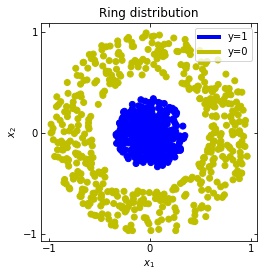
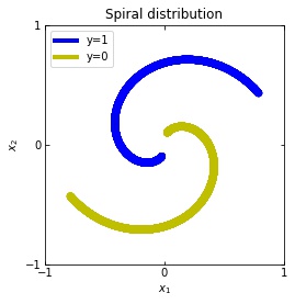 Plot of the ring and spiral distribution.
And let’s put into practice what we have learned! For that, we use the library TensorFlow [14], in which we can easy implement the Multilayer Perceptrons and Residual Neural Networks that we have defined.
We are going to look at the evolution of $x(t)$, with $x(0)$ the initial datapoint of the dataset. Remember that we have two cases
- In a multilayer perceptron, $x(t) = x_t = f^t \circ f^{t-1} \circ … \circ f^1(x)$.
- In a ResNet, $x(t)$ would be given by $x(t+1) = x(t) + f(x(t))$ that is, approximately, $\dot{x}(t) = G(x(t), t)$.
Multilayer Perceptrons
In the case of multilayer perceptrons, we choose $3$ neurons per layer. This means that we are working with points $x(t)$ in $\mathbb{R}^3$.
We train the networks, and after lots of iterations of the gradient descent method, this is what we obtain.

We see that in the final space (hidden layer 5) the blue and yellow points can be linearly separable.
However, the dynamics is far from smooth, and we see that in the final layers we seem to occupy a $2-$dimensional space rather than a $3-$dimensional one. This is because multilayer perceptrons tend to “lose information”. This type of behaviour causes that if we had increased the number of layers this architectures would be super difficult to train (we would have to try lots of times, since each time we initialize the parameters at random).
Visualizing ResNets
With ResNets we are far luckier!
Consider two neurons per layer. That is, we would be working with $x(t)$ in $\mathbb{R}^2$.
We observe that altough the spiral distribution can be classified by this neurons (the transformed space, in hidden layer $49$, makes the distribution linearly separable) this does not happen with the ring distribution!
We should be able to respond why this happens with what we have learned: since the ResNets are homeomorphisms, we would not be able to untie the tie in the ring distribution!
However, we should be able to untie it if going to a third dimension. Let’s try that.
Now we consider $3$ neurons per layer, i.e. $x(t) \in \mathbb{R}^3$.
Now both distributions can be classified. Indeed, every distribution in a plane could be in principle classified by a ResNet, since at most we would have ties of order $2$, that can be untied in a dimension $3$.
But could indeed all distributions be classified? Are the ResNets indeed such powerful approximators that we could recreate almost any dynamics out of them? Are we able to find the parameters $\theta$ (that can be seen as controls) such that all distributions can be classified? What do we gain by increasing $T$ (having more and more layers)?
Those and far more other questions arise out of this approach. And those cannot be answered easily without further research.
Results, open questions and perspectives
Noisy vs noisless data
 Representation of a more natural distribution at the left, and examples of realisations of that distribution in the right.
It seems like we almost forgot that the data is (always) noisy! What happens in that case?
Considering the distribution in the figure (that can be seen as a more “natural” ring distribution), if we only cared about moving the blue points to the top, and the yellow points to the bottom, we would have an inecessary complex dynamics, since we expect some points to be mislabelled.
We should stick to “simple dynamics”, that are the ones we expect would generalise well. But how to define “simple dynamics”?
In an optimal control approach, this has to do with adding regularization terms.
Moreover, Weinan E. et al [2] propose the approach of considering, instead of our points $x(t)$ as objects of study for the dynamics, the probabilty distribution, and so recasting the control as a mean field optimal control. With this approach, some we gain some insight into the problem of generalization.
This has to do with the idea that indeed what the Neural Networks take as inputs are probabilty distributions, and the dynamics should be focused on those. In here theories such as transportation theory try to give some insight into happens when consider the more general problem of Deep Learning: one in which we have noise.
Complexity and control of Neural Networks
We also do not know what happens when increasing the number of layers. Why increasing the number of layers is better?
In practice, having more layers (working in the so called overparametrization regime) seems to perform better in training. Our group indeed gave some insight in that direction [15] by connecting this problems with the turnpike phenomenon [16].
Regarding optimality, it is not easy to define, since we have multiple possible solutions to the same problem. That is, there are multiple dynamics that can make an initial distribution linearly separable.
 Dynamics given by a ResNet with 3 neurons per layer, with two different initializations.
The question is again: if there is a family of dynamics that solve the classification problem, which ones out of that family are optimal?
It also seems that one should take into account some problem of stochastic control, since the parameters $\theta$ are initialized at random, and different initializations give different results in practice. Moreover, the stochastic gradient descent, which is widely used, introduces some randomness to our problem. This indicates that Deep Learning is by no means a classical control problem.
Conclusions
Altough the problem of Deep Learning is not yet resolved, we have made a some very interesting equivalences:
- The problem of approximation in Deep Learning is now the problem of how is the space of possible dynamics? In the case of multilayer perceptrons, we can make use of discrete dynamical systems to solve that, or characterize their complexity; and in the case of ResNets, papers such at the one by Q. Li et. deals with that question [7].
- The problem of optimization is the problem of finding the best weights $\theta$, that can be recasted as controls. That is, is a problem of optimal control, and we should be able to use our knowledge of optimal control (for example, the method of succesive approximations) in this direction.
- The generalization problem can be understood by consdering the control of the whole probability distribution, instead of the risk minimization problem [2].
All in all, there is still lot of work to do to understand Deep Learning.
However, the presented approaches have been giving very interesting results in the recent years, and everything indicates that they will continue to do so.
References
[1] J. Behrmann, W. Grathwohl, R. T. Q. Chen, D. Duvenaud, J. Jacobsen (2018). Invertible Residual Networks arxiv
[2] Weinan E, Jiequn Han, Qianxiao Li, (2018). A Mean-Field Optimal Control Formulation of Deep Learning. volume 6. Research in the Mathematical Sciences. paper
[4] B. Hanin, (2018). Which Neural Net Architectures Give Rise to Exploding and Vanishing Gradients? arxiv
[5] C. Olah, Neural Networks, Manifolds and Topology . blog post
[6] G. Naitzat, A. Zhitnikov, L-H. Lim, (2020). Topology of Deep Neural Networks arxiv
[7] Q. Li, T. Lin, Z. Shen, (2019). Deep Learning via Dynamical Systems: An Approximation Perspective arxiv
[8] B. Geshkovski, The interplay of control and deep learning . blog post
[9] C. Fefferman, S. Mitter, H. Narayanan, Testing the manifold hypothesis . pdf
[10] R. T. Q. Chen, Y. Rubanova, J. Bettencourt, D. Duvenaud, (2018). Neural Ordinary Differential Equations arxiv
[11] G. Cybenko. Approximation by Superpositions of a Sigmoidal Function pdf
[12] Weinan E, Chao Ma, S. Wojtowytsch, L. Wu. Towards a Mathematical Understanding of Neural Network-Based Machine Learning_ what we know and what we don’t. arxiv
[14] Introduction to TensorFlow . tutorial
[15] C. Esteve, B. Geshkovski, D. Pighin, E. Zuazua Large-time asymptotics in deep learning . arxiv
[16] Turnpike in a Nutshell . Collection of talks