We describe here a Finite Element algorithm for the approximation of the one-dimensional fractional Laplacian $(-d_x^2)^s$ on the interval $(-L,L)$ , $L>0$ and for the numerical resolution of the following fractional Poisson equation

$\begin{equation}\label{Fl_Poisson} \begin{cases} (-d_x^2)^s u = f, & x\in (-L,L) \\ u = 0, & x\in(-L^L)^c=: \mathbb{R}\setminus (-L,L.) \end{cases} \end{equation}$

This algorithm has also been emploied in [2,3] for the numerical controllability of fractional parabolic problems (see our previous entries in the DyCon Blog, WP3_P0001 and WP3_P0022).

We recall that the fractional Laplacian is defined, for all $s\in(0,1)$ and any function $u$ regular enough, as the following singular integral

$(-d_x^2)^s u(x) := c_s \,P.V.\,\int_{\mathbb{R}} \frac{u(x)-u(y)}{|x-y|^{1+2s}}\,dy,$

with $c_s$ an explicit normalization constant given by

$c_s = \frac{s2^{2s}\Gamma\left(\frac{1+2s}{2}\right)}{\sqrt{\pi}\Gamma(1-s)},$

$\Gamma$ being the usual Euler Gamma function.

The starting point of the FE method is the definition of a bilinear form associated to the fractional Laplace operator $(-d_x^2)^s$ and the introduction of the variational formulation corresponding to the elliptic problem $\eqref{Fl_Poisson}$ .

This variational formulation is given as follows: find $u\in H_0^s(-L,L)$ such that the identity

$\begin{equation}\label{variational} a(u,v) = \int_{-L}^L fv\,dx \end{equation}$

is satisfied for any function $v\in H_0^s(-L,L)$ . In $\eqref{variational}$ , with $H_0^s(-L,L)$ we indicate the space

$H_0^s(-L,L):=\Big\{ u\in H^s(\mathbb{R})\;:\; u=0\;in\; (-L,L)^c\Big\},$

$H^s(\mathbb{R})$ being the usual fractional Sobolev space. Moreover, the bilinear form

$a: H_0^s(-L,L)\times H_0^s(-L,L)\to \mathbb{R}$

is defined as

$a(u,v) = \frac{c_s}{2}\int_{\mathbb{R}}\int_{\mathbb{R}} \frac{(u(x)-u(y))(v(x)-v(y))}{|x-y|^{1+2s}}\,dxdy.$

Let us describe how, starting from the above bilinear form, we can obtain our FE approximation. For simplicity, in what follows we will take $L=1$ , although the methodology remains the same for any real $L>0$ .

Let us take a uniform partition of the interval $(-1,1)$ as follows:

$-1 = x_0<x_1<\ldots <x_i<x_{i+1}<\ldots<x_{N+1}=1\,,$

with $x_{i+1}=x_i+h$ , $i=0,\ldots N$ . We call $\mathfrak{M}$ the mesh composed by the points ${x_i\,:\, i=1,\ldots,N}$ , while the set of the boundary points is denoted $\partial\mathfrak{M}:={x_0,x_{N+1}}$ .

Now, define $K_i:=[x_i,x_{i+1}]$ and consider the discrete space

$\begin{equation}\label{Vh} V_h :=\Big\{v_h\in H_0^s(-1,1)\,\big|\, \left. v_h\,\right|_{K_i}\in \mathcal{P}^1\Big\}, \end{equation}$

where $\mathcal{P}^1$ is the space of the continuous and piece-wise linear functions. Hence, we approximate $\eqref{variational}$ with the following discrete problem: find $u_h\in V_h$ such that

$\frac{c_s}{2} \int_{\mathbb{R}}\int_{\mathbb{R}}\frac{(u_h(x)-u_h(y))(v_h(x)-v_h(y))}{|x-y|^{1+2s}}\,dxdy = \int_{-1}^1 fv_h\,dx,$

for all $v_h\in V_h$ . If now we indicate with

$\big\{\phi_i\big\}_{i=1}^N$

a basis of $V_h$ , it will be sufficient that the above equality is satisfied for all the functions of the basis, since any element of $V_h$ is a linear combination of them. Therefore the problem takes the following form

$\begin{equation}\label{WFD} \frac{c_s}{2} \int_{\mathbb{R}}\int_{\mathbb{R}}\frac{(u_h(x)-u_h(y))(\phi_i(x)-\phi_i(y))}{|x-y|^{1+2s}}\,dxdy = \int_{-1}^1 fv_h\,dx,\;\;\; i=1,\ldots,N. \end{equation}$

Clearly, since $u_h\in V_h$ , we have $u_h(x) = \sum_{j=1}^N u_j\phi_j(x)$ , where the coefficients $u_j$ are, a priori, unknown. In this way, $\eqref{WFD}$ is reduced to solve the linear system $\mathcal A_h u=F$ , where the stiffness matrix $\mathcal A_h\in \mathbb{R}^{N\times N}$ has components

$\begin{equation}\label{stiffness_nc} a_{i,j}=\frac{c_s}{2} \int_{\mathbb{R}}\int_{\mathbb{R}}\frac{(\phi_i(x)-\phi_i(y))(\phi_j(x)-\phi_j(y))}{|x-y|^{1+2s}}\,dxdy, \end{equation}$

while the vector $F\in\mathbb{R}^N$ is given by $F=(F_1,\ldots,F_N)$ with

$F_i = \langle f,\phi_i\rangle_{L^2(-1,1)} = \int_{-1}^1 f\phi_i\,dx,\;\;\; i=1,\ldots,N.$

Moreover, the basis

$\big\{\phi_i\big\}_{i=1}^N$

that we will employ is the classical one in which each $\phi_i$ is the tent function with $supp(\phi_i)=(x_{i-1},x_{i+1})$ and verifying $\phi_i(x_j)=\delta_{i,j}$ . In particular, for $x\in{x_{i-1},x_i,x_{i+1}}$ the $i^{th}$ function of the basis is explicitly defined as (see Figure 1)

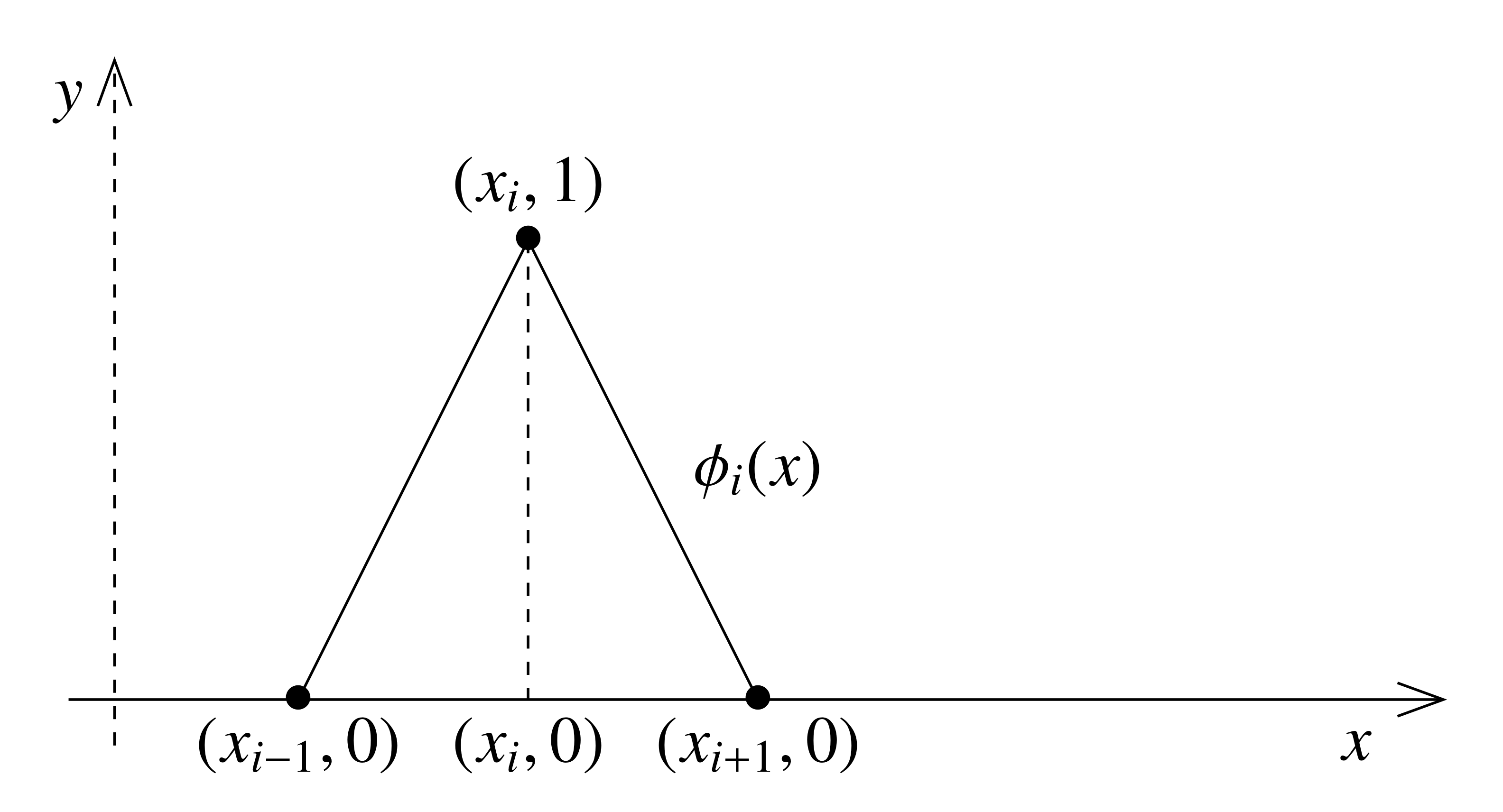
$\begin{equation}\label{basis_fun} \phi_i(x)= 1-\frac{|x-x_i|}{h}. \end{equation}$

Figure 1. Basis function $\phi_i$ on its support $(x_{i-1},x_{i+1})$ .

We now start building the stiffness matrix $\mathcal A_h$ approximating the fractional Laplacian. This will be done in three steps, since the values of the matrix can be computed differentiating among three well defined regions: the upper triangle, corresponding to $j\geq i+2$ , the upper diagonal corresponding to $j=i+1$ and the diagonal, corresponding to $j=i$ . In each of these regions the intersections among the support of the basis functions are different, thus generating different values of the bilinear form.

We present below an abridged explanation of how to compute the entries of $\mathcal{A}_h$ . Complete details may be found in [2].

Step 1: $j\geq i+2$

In this case we have $supp(\phi_i)\cap supp(\phi_j) =\emptyset$ (see also Figure 2). Hence, $\eqref{stiffness_nc}$ is reduced to computing only the integral

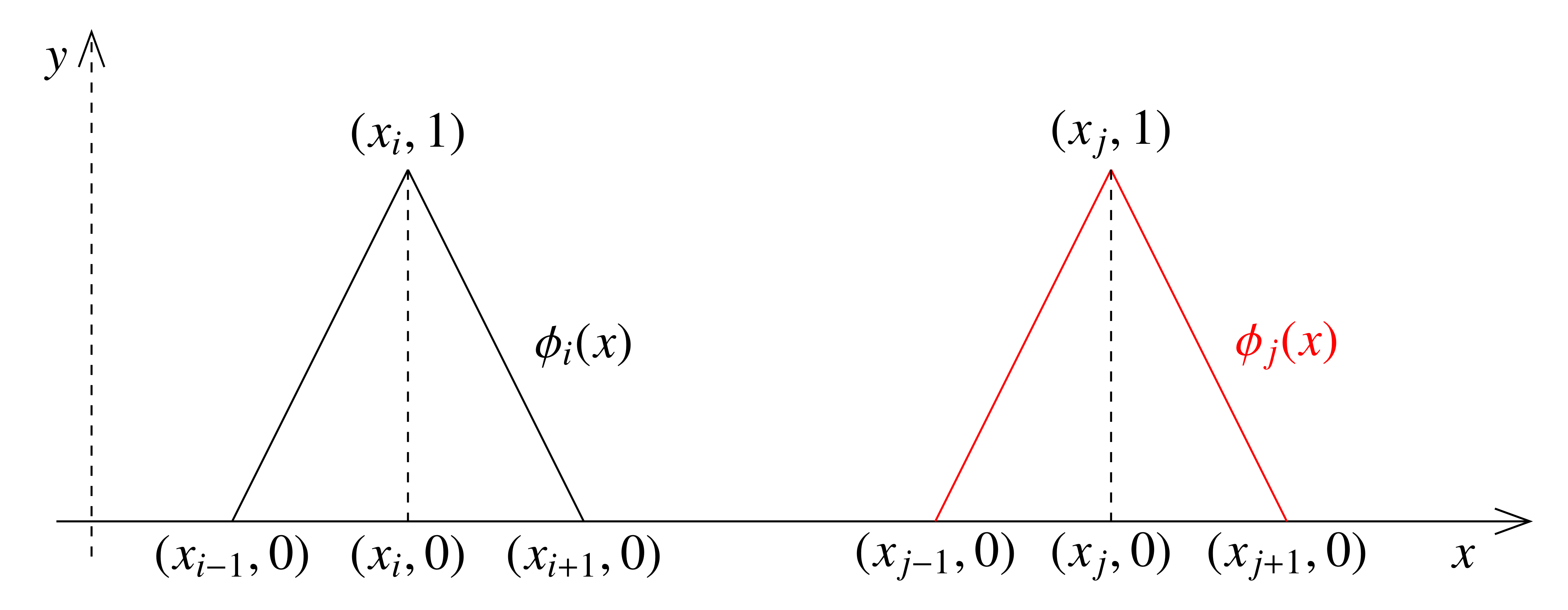
$\begin{equation}\label{elem_noint_app} a_{i,j}=-2 \int_{x_{j-1}}^{x_{j+1}}\int_{x_{i-1}}^{x_{i+1}}\frac{\phi_i(x)\phi_j(y)}{|x-y|^{1+2s}}\,dxdy. \end{equation}$

Figure 2. Basis functions $\phi_i(x)$ and $\phi_j(x)$ for $j\geq i + 1$ . The supports are disjoint.

Taking into account the definition of the basis function $\eqref{basis_fun}$ , the integral $\eqref{elem_noint_app}$ becomes

$a_{i,j}=-2 \int_{x_{j-1}}^{x_{j+1}}\int_{x_{i-1}}^{x_{i+1}}\frac{\left(1-\frac{|x-x_i|}{h}\right)\left(1-\frac{|y-x_j|}{h}\right)}{|x-y|^{1+2s}}\,dxdy.$

Let us introduce the following change of variables:

$\begin{equation}\label{CV} \frac{x-x_i}{h}=\hat{x},\;\;\; \frac{y-x_j}{h}=\hat{y}. \end{equation}$

Then, rewriting (with some abuse of notations since there is no possibility of confusion) $\hat{x}=x$ and $\hat{y}=y$ , we get

$a_{i,j}=-2h^{1-2s} \int_{-1}^1\int_{-1}^1\frac{(1-|x\,|\,)(1-|y\,|\,)}{|x-y+i-j\,|^{1+2s}}\,dxdy.$

This integral can be computed explicitly, and we obtain

$a_{i,j} = - h^{1-2s}\,\frac{4(k+1)^{3-2s} + 4(k-1)^{3-2s}-6k^{3-2s}-(k+2)^{3-2s}-(k-2)^{3-2s}}{2s(1-2s)(1-s)(3-2s)}.$

Notice that, when $s=1/2$ , both the numerator and the denominator of the expression above are zero. In this case, the value of $a_{i,j}$ can be obtained by taking the limit $s\to 1/2$ and we get

$\begin{array}{l} a_{i,j} &= -4 (k+1)^2\log(k+1) -4(k-1)^2\log(k-1)+6k^2\log(k) \\[10pt] &+(k+2)^2\log(k+2) +\;(k-2)^2\log(k-2) \end{array}$

if $k\neq 2$ and

$a_{i,i+2} = 56\ln(2)-36\ln(3).$

Step 2: $j= i+1$

This is the most cumbersome case, since it is the one with the most interactions between the basis functions (see Figure 3).

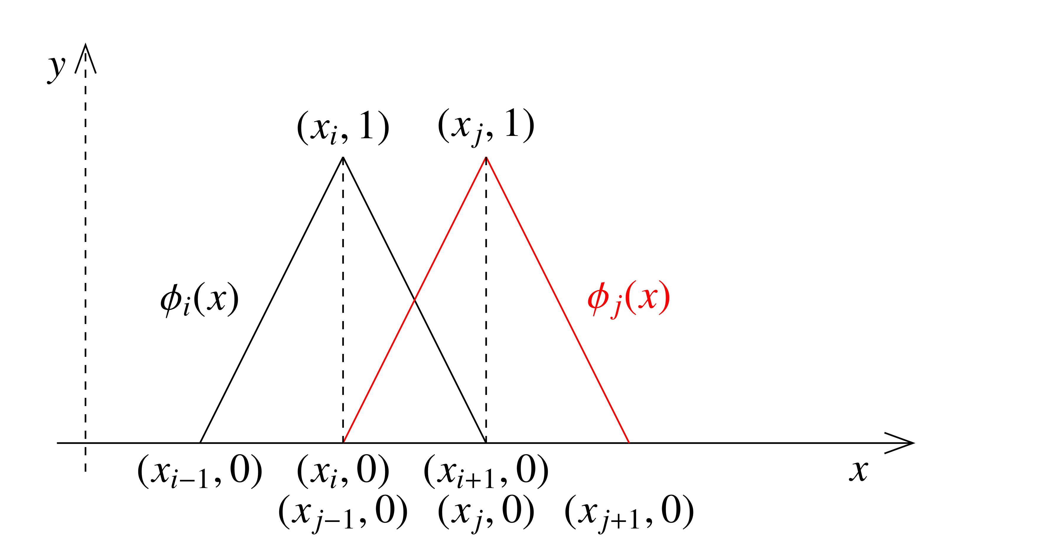
Figure 3. Basis functions $\phi_i(x)$ and $\phi_{i+1}(x)$ . In this case, the intersection of the supports is the interval $[x_i,x_{i+1}]$ .

Using the symmetry of the integral with respect to the bisector $y=x$ , we have

$\begin{array}{ll} a_{i,i+1} &= \displaystyle\int_{\mathbb{R}}\int_{\mathbb{R}}\frac{(\phi_i(x)-\phi_i(y))(\phi_{i+1}(x)-\phi_{i+1}(y))}{|x-y|^{1+2s}}\,dxdy \\[15pt] &= \displaystyle\int_{x_{i+1}}^{+\infty}\int_{x_{i+1}}^{+\infty} \ldots\,dxdy + 2\int_{x_{i+1}}^{+\infty}\int_{x_i}^{x_{i+1}} \ldots\,dxdy + 2\int_{x_{i+1}}^{+\infty}\int_{-\infty}^{x_i} \ldots\,dxdy \\[15pt] &\quad + \displaystyle\int_{x_i}^{x_{i+1}}\int_{x_i}^{x_{i+1}} \ldots\,dxdy + 2\int_{x_i}^{x_{i+1}}\int_{-\infty}^{x_i} \ldots\,dxdy + \int_{-\infty}^{x_i}\int_{-\infty}^{x_i} \ldots\,dxdy \\[15pt] &:= Q_1 + Q_2 + Q_3 + Q_4 + Q_5 + Q_6. \end{array}$

Also in this case, the terms $Q_i$ , $i=1,\ldots,6$ , can be computed explicitely, by noticing also the following facts:

$Q_1=Q_6=0$ since $\phi_i = 0$ on the domain of integration.
$Q_2=Q_5$ due to symmetry.

Then, the elements $a_{i,i+1}$ are given by the sum $2Q_2+Q_3+Q_4$ and we have

$a_{i,i+1} = \begin{cases} \displaystyle h^{1-2s}\frac{3^{3-2s}-2^{5-2s}+7}{2s(1-2s)(1-s)(3-2s)}, & \displaystyle s\neq \frac{1}{2} \\[15pt] 9\ln 3-16\ln 2, & \displaystyle s=\frac{1}{2}. \end{cases}$

Step 3: $j= i$

As a last step, we fill the diagonal of the matrix $\mathcal A_h$ , which collects the values corresponding to $\phi_i(x)=\phi_j(x)$ (see Figure 4).

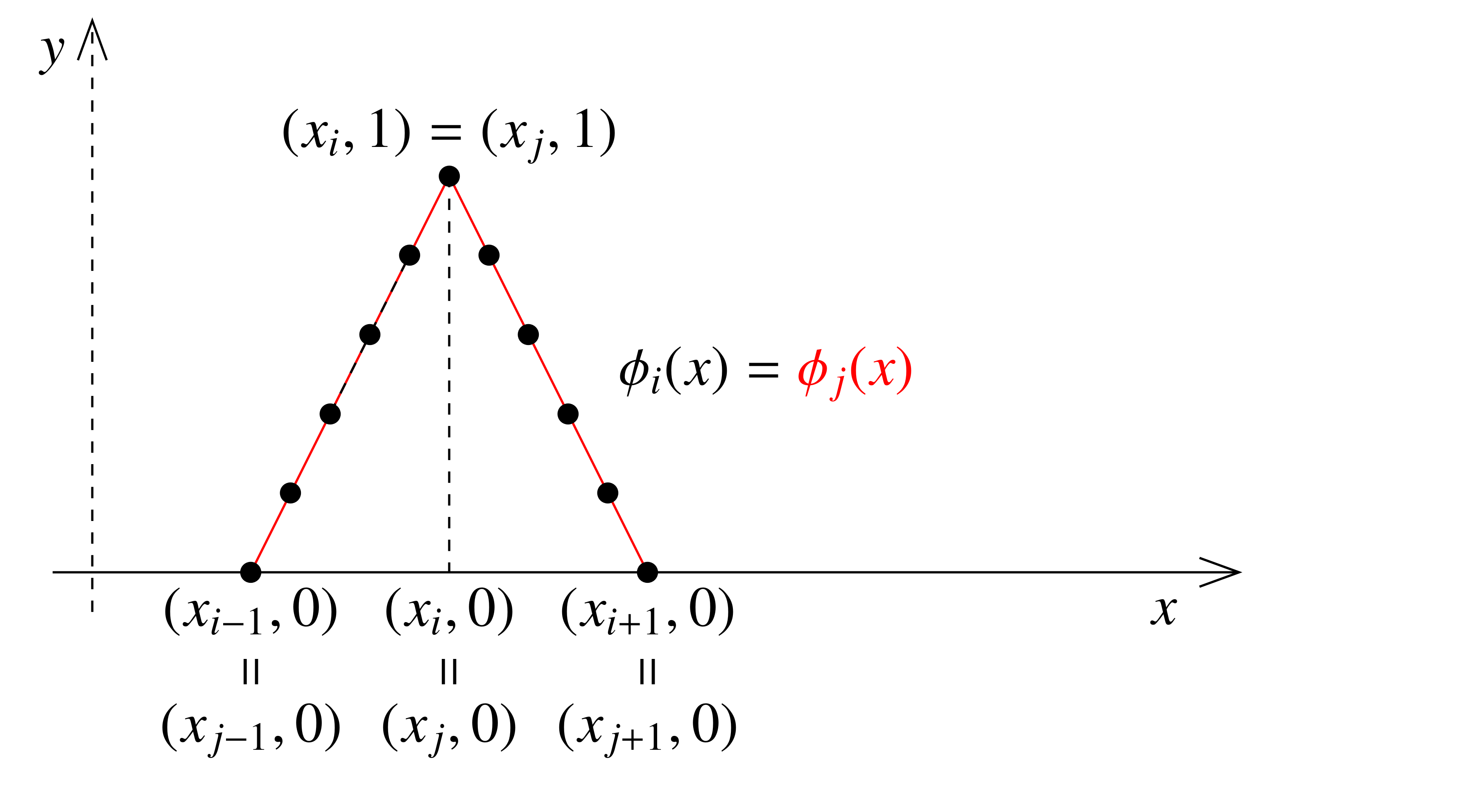
Figure 4. Basis functions $\phi_i(x)=\phi_j(x)$ .

In this case, we have

$\begin{array}{ll} a_{i,i} &= \displaystyle\int_{\mathbb{R}}\int_{\mathbb{R}}\frac{(\phi_i(x)-\phi_i(y))^2}{|x-y|^{1+2s}}\,dxdy \\[15pt] & = \displaystyle\int_{x_{i+1}}^{+\infty}\int_{x_{i+1}}^{+\infty} \ldots\,dxdy + 2\int_{x_{i+1}}^{+\infty}\int_{x_{i-1}}^{x_{i+1}} \ldots\,dxdy + \int_{x_{i+1}}^{+\infty}\int_{-\infty}^{x_{i-1}} \ldots\,dxdy \\[15pt] & \quad\displaystyle+ \int_{x_{i-1}}^{x_{i+1}}\int_{x_{i-1}}^{x_{i+1}} \ldots\,dxdy + 2\int_{-\infty}^{x_{i-1}}\int_{x_{i-1}}^{x_{i+1}} \ldots\,dxdy + + \int_{-\infty}^{x_{i-1}}\int_{x{i+1}}^{+\infty} \ldots\,dxdy \\[15pt] & \quad\displaystyle + \int_{-\infty}^{x_{i-1}}\int_{-\infty}^{x_{i-1}} \ldots\,dxdy := R_1 + R_2 + R_3 + R_4 + R_5 + R_6 + R_7. \end{array}$

Once again, the terms $R_i$ , $i=1,\ldots,7$ can be computed explicitely, by taking also into account that $R_1=R_3=R_6=R_7=0$ because the corresponding integration domains are all away from the support of the basis functions.

The result of these computations gives the values

$a_{i,i} = \begin{cases} \displaystyle h^{1-2s}\,\frac{2^{3-2s}-4}{s(1-2s)(1-s)(3-2s)}, & \displaystyle s\neq\frac{1}{2} \\ \\ 8\ln 2, & \displaystyle s=\frac{1}{2}. \end{cases}$

Step 4: building of $\mathcal A_h$

Summarizing, we have the following values for the elements of the stiffness matrix $\mathcal{A}_h$ : for $s\neq 1/2$

$a_{i,j} = -h^{1-2s} \begin{cases} \displaystyle \,\frac{4(k+1)^{3-2s} + 4(k-1)^{3-2s}-6k^{3-2s}-(k+2)^{3-2s}-(k-2)^{3-2s}}{2s(1-2s)(1-s)(3-2s)}, & \displaystyle k=j-i,\,k\geq 2 \\ \\ \displaystyle\frac{3^{3-2s}-2^{5-2s}+7}{2s(1-2s)(1-s)(3-2s)}, & \displaystyle j=i+1 \\ \\ \displaystyle\frac{2^{3-2s}-4}{s(1-2s)(1-s)(3-2s)}, & \displaystyle j=i. \end{cases}$

For $s=1/2$ , instead, we have

$a_{i,j} = \begin{cases} -4(j-i+1)^2\log(j-i+1)-4(j-i-1)^2\log(j-i-1) \\ \;\;\;+6(j-i)^2\log(j-i)+(j-i+2)^2\log(j-i+2)+(j-i-2)^2\log(j-i-2), & \displaystyle j> i+2 \\ \\ 56\ln(2)-36\ln(3), & \displaystyle j= i+2. \\ \\ \displaystyle 9\ln 3-16\ln 2, & \displaystyle j=i+1 \\ \\ \displaystyle 8\ln 2, & \displaystyle j=i. \end{cases}$

Numerical results

We present the numerical simulations corresponding to the algorithm previously described.

First of all, we test numerically the accuracy of our method for the resolution of the elliptic equation $\eqref{Fl_Poisson}$ by applying it to the following problem

$\begin{equation}\label{poisson} \begin{cases} (-d_x^2)^s u = 1, & x\in(-1,1) \\ u\equiv 0, & x\in(-1,1)^c. \end{cases} \end{equation}$

In this particular case, the unique solution $u$ can be computed exactly and it is given by

$\begin{equation}\label{real_sol} u(x)=\frac{2^{-2s}\sqrt{\pi}}{\Gamma\left(\frac{1+2s}{2}\right)\Gamma(1+s)}\Big(1-x^{\,2}\Big)^s\cdot\chi_{(-1,1)}, \end{equation}$

where $\chi_{(-1,1)}$ indicates the characteristic function of the interval $(-1,1)$ .

The solution of $\eqref{poisson}$ in the case $s=0.1$ and $N=50$ is computed with the following script which emploies the function FEFractionalLaplacian.m ginving the FE discretization of $(-d_x^2)^s$ .

s = 0.1;
N = 50;
L = 1;

x = linspace(-L,L,N+2);
x = x(2:end-1);
h = x(2)-x(1);

f = @(x) 1+0*x;
Phi = @(x) 1-abs(x);

F = zeros(N,1);

for i=1:N
    xx = linspace(x(i)-h,x(i)+h,N+1);
    xx = 0.5*(xx(2:end)+xx(1:end-1));
    B1 = f(xx).*(Phi((xx-x(i))/h));
    F(i) = ((2*h)/N)*sum(B1); 
end

A = FEFractionalLaplacian(s,L,N);
sol = A\F;

In Figure 5, we show a comparison for different values of $s$ between the exact solution $\eqref{real_sol}$ and the computed numerical approximation.

Figure 5. Real and numerical solution.

One can notice that when $s=0.1$ (and also for other small values of s), the computed solution is to a certain extent different from the exact solution. Notwithstanding, it is well-known that the notion of trace is not defined for the spaces $H^s(-1,1)$ with $s\leq 1/2$ . Hence, it is somehow natural that we cannot expect a point-wise convergence in this case.

Furthermore, the accuracy of our algorithm is validated by a simple error analysis.

The computation of the error in the space $H_0^s(-1,1)$ can be readily done by using the definition of the bilinear form, namely

$\|u-u_h\|_{H_0^s(-1,1)}^2 =a(u-u_h,u-u_h) =a(u,u-u_h) =\int_{-1}^1f(x)\left(u(x)-u_h(x)\right)dx$

where have used the orthogonality condition $a(v_h,u-u_h)=0$ for all $v_h \in V_h$ .

For this particular test, since $f\equiv 1$ in $(-1,1)$ , the problem is therefore reduced to

$\|u-u_h\|_{H^s_0(-1,1)}=\left(\int_{-1}^1\left( u(x)-u_h(x) \right)\,dx\right)^{1/2}$

where the right-hand side can be easily computed, since we have the closed formula

$\int_{-1}^1u\,dx= \frac{\pi}{2^{2s}\Gamma(s+\frac{1}{2})\Gamma(s+\frac{3}{2})}$

and the term corresponding to $\int_{-1}^1u_h$ can be carried out numerically. Moreover, we have the following convergence result.

Theorem [2] For the solution $u$ of $\eqref{WFD}$ and its FE approximation $u_h$ given by $\eqref{WFD}$ , if $h$ is sufficiently small, the following estimates hold

$\begin{array}{ll} \|u-u_h\|_{H^s_0(-1,1)}\leq \mathcal{C} h^{1/2}|\!\ln h|\,\|f\|_{C^{1/2-s}(-1,1)}, &\text{if}\quad s<1/2, \\[15pt] \|u-u_h\|_{H^s_0(-1,1)}\leq \mathcal{C} h^{1/2} |\!\ln h|\, \|f\|_{L^\infty(-1,1)},&\text{if}\quad s=1/2 \\[15pt] \displaystyle\|u-u_h\|_{H^s_0(-1,1)}\leq \tfrac{\mathcal{C}}{2s-1} h^{1/2} \sqrt{|\!\ln h|}\, \|f\|_{C^\beta(-1,1)},& \text{if} \quad s>1/2,\;\;\beta>0 \end{array}$

where $\mathcal{C}$ is a positive constant not depending on $h$ .

In Figure 6, we present the computational errors evaluated for different values of $s$ and $h$ , which can be obtained with the following function.

function [h,e] = error_fl(s,N)

x = linspace(-1,1,N+2);
x = x(2:end-1);
h = x(2)-x(1);

f = @(x) 1+0*x;
Phi = @(x) 1-abs(x);

F = zeros(N,1);

for i = 1:N
    xx = linspace(x(i)-h,x(i)+h,N+1);
    xx = 0.5*(xx(2:end)+xx(1:end-1));
    B1 = f(xx).*(Phi((xx-x(i))/h));
    F(i) = ((2*h)/N)*sum(B1); 
end

A = FEFractionalLaplacian(s,1,N);
sol = A\F;
val = pi/(2^(2*s)*gamma(s+0.5)*gamma(s+1.5));
valnum = h*sum(sol);
e = sqrt(val-valnum);

Figure 6. Computational error in logarithmic scale in terms for different values of $s$ .

The rates of convergence shown are of order (in $h$ ) of $1/2$ , and this convergence rate is maintained also for small values of $s$ . This confirms the accuracy of our approximation. In particular, the behavior shown in Figure 6 is not in contrast with the known theoretical results.

References

[1] G. Acosta, F. Bersetche and J. P. Borthagaray, A short FE implementation for a 2d homogeneous Dirichlet problem of a Fractional Laplacian. Comput. Math. Appl., Vol. 74, No. 4 (2017), pp. 784-816.

[2] U. Biccari and V. Hernández-Santamarı́a, Controllability of a one-dimensional fractional heat equation: theoretical and numerical aspects. IMA J. Math. Control. Inf, to appear, 2018.

[3] U. Biccari, M. Warma and E. Zuazua, Controllability of the one-dimensional fractional heat equation under positivity constraints. Submitted.

Work Packages ≻ Models involving memory terms and hybrid PDE+ODE systems ≻

Finite Element approximation of the one-dimensional fractional Laplacian

Step 1: $j\geq i+2$

Step 2: $j= i+1$

Step 3: $j= i$

Step 4: building of $\mathcal A_h$

Numerical results

References

Related Posts

Moving control strategy for memory-type equations

Simulation of Fractional Heat Equation

Optimal Control of the Fokker-Planck Equation with CasADi

Numerical simulation of nonlinear Population Dynamics Structuring by age and Spatial diffusion

Step 1: j≥i+2j\geq i+2

Step 2: j=i+1j= i+1

Step 3: j=ij= i

Step 4: building of Ah\mathcal A_h

Numerical results

References

Related Posts

Moving control strategy for memory-type equations

Simulation of Fractional Heat Equation

Optimal Control of the Fokker-Planck Equation with CasADi

Numerical simulation of nonlinear Population Dynamics Structuring by age and Spatial diffusion

Step 1: $j\geq i+2$

Step 2: $j= i+1$

Step 3: $j= i$

Step 4: building of $\mathcal A_h$