The Dirichlet-Neumann iteration for two coupled heterogeneous heat equations

Download Code

The time dependent transmission problem is as follows, where we consider a domain $\Omega \subset \mathbb{R}^2$ which is cut into two subdomains $\Omega_1 \cup \Omega_2 = \Omega$ with transmission conditions at the interface $\Gamma = \Omega_1 \cap \Omega_2$:

$$\begin{align} \begin{split} & \alpha_m \frac{\partial u_m(\textbf{x},t)}{\partial t} - \nabla \cdot (\lambda_m \nabla u_m(\textbf{x},t)) = 0,\ \ t \in [t_0, t_f], \ \ \textbf{x} \in \Omega_m \subset \mathbb{R}^2, \\ & u_m(\textbf{x},t) = 0, \ \ t \in [t_0, t_f], \ \ \textbf{x} \in \partial \Omega_m \backslash \Gamma, \\ & u_1(\textbf{x},t) = u_2(\textbf{x},t), \ \ \textbf{x} \in \Gamma, \\ & \lambda_2 \frac{\partial u_2(\textbf{x},t)}{\partial \textbf{n}_2} = -\lambda_1 \frac{\partial u_1(\textbf{x},t)}{\partial \textbf{n}_1}, \ \ \textbf{x} \in \Gamma, \\ & u_m(\textbf{x},0) = u_m^0(\textbf{x}), \ \ \textbf{x} \in \Omega_m, \end{split} \end{align}$$

where $\textbf{n}_m$ is the outward normal to $\Omega_m$ for $m=1,2$.

The constants $\lambda_1$ and $\lambda_2$ describe the thermal conductivities of the materials on $\Omega_1$ and $\Omega_2$ respectively. $D_1$ and $D_2$ represent the thermal diffusivities of the materials and they are defined by

$$\begin{align} D_m = \frac{\lambda_m}{\alpha_m}, \ \ \mbox{with} \ \ \alpha_m = \rho_m c_{p_m} \end{align}$$

where $\rho_m$ represents the density and $c_{p_m}$ the heat capacity of the material placed in $\Omega_m$, $m=1,2$.

DISCRETIZATION

Let $u_I^{(1)}$ and $u_I^{(2)}$ correspond to the unknowns on $\Omega_1$ and $\Omega_2$ respectively and $u_{\Gamma}$ correspond to the unknows at the interface $\Gamma$, then the compact 2D finite difference (FD) formulation on equidistant meshes of (1) for the vector of unknowns

$$\textbf{u} = (\textbf{u}_I^{(1)}, \textbf{u}_I^{(2)}, \textbf{u}_{\Gamma})^T$$

will be

$$\begin{equation} \tilde{\textbf{M}} \dot{\textbf{u}} - \tilde{\textbf{A}} \textbf{u} = 0 \ \ \mbox{where} \ \ \tilde{\textbf{M}} = \left( \begin{array}{ccc} \textbf{M}_1 & \textbf{0} & \textbf{M}_{I \Gamma}^{(1)} \\ \textbf{0} & \textbf{M}_2 & \textbf{M}_{I \Gamma}^{(2)} \\ \textbf{M}_{\Gamma I}^{(1)} & \textbf{M}_{\Gamma I}^{(2)} & \textbf{M}_{\Gamma \Gamma}^{(1)} + \textbf{M}_{\Gamma \Gamma}^{(2)} \end{array} \right), \ \ \tilde{\textbf{A}} = \left( \begin{array}{ccc} \textbf{A}_1 & \textbf{0} & \textbf{A}_{I \Gamma}^{(1)} \\ \textbf{0} & \textbf{A}_2 & \textbf{A}_{I \Gamma}^{(2)} \\ \textbf{A}_{\Gamma I}^{(1)} & \textbf{A}_{\Gamma I}^{(2)} & -\textbf{A}_{\Gamma \Gamma}^{(1)} - \textbf{A}_{\Gamma \Gamma}^{(2)} \end{array} \right), \end{equation}$$

for the mass matrices $M_m$, $M_{\Gamma \Gamma}^{(m)}$, $M_{I \Gamma}^{(m)}$, $M_{\Gamma I}^{(m)}$ and the stiffness matrices

$$\textbf{A}_m, \textbf{A}_{\Gamma \Gamma}^{(m)}, \textbf{A}_{I \Gamma}^{(m)}, \textbf{A}_{\Gamma I}^{(m)}$$

for $m=1,2$.

Applying the implicit Euler method with time step $\Delta t$ to the system (3), we get for the vector of unknowns

$$u^{n+1} = (u_I^{(1),n+1}, u_I^{(2),n+1}, u_{\Gamma}^{n+1})^T$$ $$\begin{equation} \textbf{A} \textbf{u}^{n+1} = \tilde{\textbf{M}} \textbf{u}^n \ \ \mbox{where} \ \ \textbf{A} = \tilde{\textbf{M}} - \Delta t \tilde{\textbf{A}}. \end{equation}$$

DIRICHLET-NEUMANN ITERATION

We now employ a standard Dirichlet-Neumann iteration to solve the discrete system (4), getting in the $k$-th iteration the two equation systems

$$\begin{equation} (\textbf{M}_1 - \Delta t \textbf{A}_1) \textbf{u}_I^{(1),n+1,k+1} = -(\textbf{M}_{I \Gamma}^{(1)} - \Delta t \textbf{A}_{I \Gamma}^{(1)}) \textbf{u}_{\Gamma}^{n+1,k} + \textbf{M}_1 \textbf{u}_I^{(1),n} + \textbf{M}_{I \Gamma}^{(1)} \textbf{u}_{\Gamma}^n, \end{equation}$$ $$\begin{equation} \hat{\textbf{A}} \hat{\textbf{u}}^{k+1} = \hat{\textbf{M}} \textbf{u}^n - \textbf{b}^k, \end{equation}$$

to be solved in succession. Here,

$$\begin{equation} \begin{split} \hat{\textbf{A}} = \left( \begin{array}{cc} \textbf{M}_2 - \Delta t \textbf{A}_2 & \textbf{M}_{I \Gamma}^{(2)} - \Delta t \textbf{A}_{I \Gamma}^{(2)} \\ \textbf{M}_{\Gamma I}^{(2)} - \Delta t \textbf{A}_{\Gamma I}^{(2)} & \textbf{M}_{\Gamma \Gamma}^{(2)} + \Delta t \textbf{A}_{\Gamma \Gamma}^{(2)} \end{array} \right), \ \ \hat{\textbf{M}} = \left( \begin{array}{ccc} \textbf{0} & \textbf{M}_2 & \textbf{M}_{I \Gamma}^{(2)} \\ \textbf{M}_{\Gamma I}^{(1)} & \textbf{M}_{\Gamma I}^{(2)} & \textbf{M}_{\Gamma \Gamma}^{(1)} + \textbf{M}_{\Gamma \Gamma}^{(2)} \end{array} \right) \ \ \mbox{and} \\ \textbf{b}^k = \left( \begin{array}{c} \textbf{0} \\ (\textbf{M}_{\Gamma I}^{(1)} - \Delta t \textbf{A}_{\Gamma I}^{(1)}) \textbf{u}_I^{(1),n+1,k+1} + (\textbf{M}_{\Gamma \Gamma}^{(1)} + \Delta t \textbf{A}_{\Gamma \Gamma}^{(1)}) \textbf{u}_{\Gamma}^{n+1,k} \end{array} \right), \ \ \hat{\textbf{u}}^{k+1} = \left( \begin{array}{c} \textbf{u}_I^{(2),n+1,k+1} \\ \textbf{u}_{\Gamma}^{n+1,k+1} \end{array} \right) \nonumber \end{split} \end{equation}$$

with some initial condition, here $u_{\Gamma}^{n+1,0} = u_{\Gamma}^{n}$. The iteration is terminated according to the standard criterion

$$\vert \textbf{u}_{\Gamma}^{k+1} - \textbf{u}_{\Gamma}^k \vert \leq \tau$$

where $\tau$ is a user defined tolerance.

IMPLEMENTATION

We consider here the thermal interaction between two different materials which physical properties are described by their thermal conductivities and diffusivities $\lambda_1$, $\lambda_2$ and $D_1$, $D_2$ respectively. Furthermore, we consider the non overlapping identical domains $\Omega_1 = [0,1] \times [0,1]$ and $\Omega_2 = [1,2] \times [0,1]$.

The initialization parameters look as follows:

In addition to the parameters above, other objects need to be specified before starting the iterative procedure. The space grids both in $x$-direction and $y$-direction are given to later plot the numerical solution, also the initial conditions $u_m^0(x)$, $x \in \Omega_m$ and the mass and stiffness matrices coming from the space discretization:

space grid w.r.t component x

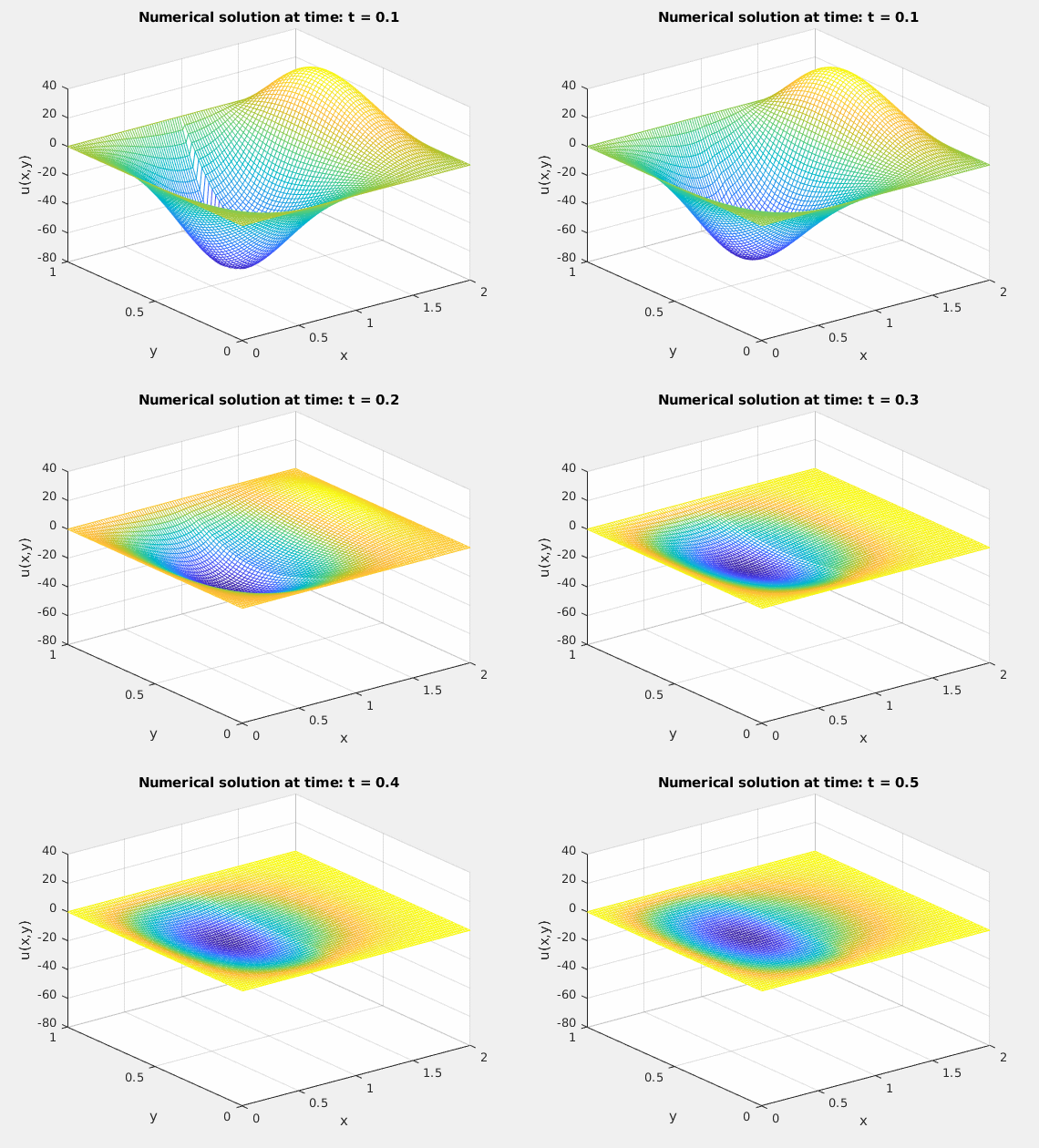
Then, the iterative procedure takes place where the equations (4) and (5) are solved alternatively on $\Omega_1$ and $\Omega_2$ respectively until convergence is achieved at each time step. The implementation is specified below:

---