Download Code
Background and motivation
We consider the initial-value problem for a Hamilton-Jacobi equation of the form
where $u_0\in C^{0,1}(\mathbb{R}^n)$ and the Hamiltonian $H: \mathbb{R}^n\rightarrow\mathbb{R}$ is assumed to satisfy the following hypotheses:
Here, the unknown $u$ is a function $[0,T]\times\mathbb{R}^n\longrightarrow\mathbb{R}$,
and the inequality $H_{pp}(p)>0$ means that the Hessian matrix of $H$ at $p$ is positive definite.
The study of Hamilton-Jacobi equations
arises in the context of optimal control theory and calculus of variations,
where the value function satisfies, in a weak sense, a Hamilton-Jacobi equation.
In this context, Hamilton-Jacobi equations have applications in a wide range of fields such as
economics, physics, mathematical finance, traffic flow and geometrical optics.
Our goal in this tutorial is to study the inverse design problem associated to (HJ).
More precisely, for a given target function $u_T$ and a time horizon $T>0$,
we want to construct all the initial conditions $u_0$ such that the viscosity solution of (HJ) coincides with $u_T$ at time $T$.
The study of this problem can also be motivated by considering the following question:
Given an observation of the solution to (HJ) at time $T>0$, can we construct all the possible initial data that agree we the observation at time $T$ ?
For this purpose, for a fixed $T>0$,
we define the following nonlinear operator, which associates to any initial condition $u_0$, the function
$u(T,\cdot)$, where $u$ is the viscosity solution of (HJ):
The inverse design problem that we are considering is then reduced to, for $u_T$ and $T>0$ given,
characterize all the initial conditions $u_0$ satisfying $S_T^+ u_0 =u_T$.
Reachability of the target
The first thing one notices when addressing this problem is that not all the Lipschitz targets are reachable.
Indeed, as it is well known, the viscosity solution to (HJ) is always a semiconcave function (see [2,4]).
Therefore, an obvious necessary (but not sufficient) condition for the reachability of $u_T$ is that it must be a semiconcave function.
See Figures 1 and 2 for some examples of unreachable targets in dimension 1 and 2 respectively. Observe that, in particular, they are not semiconcave functions.
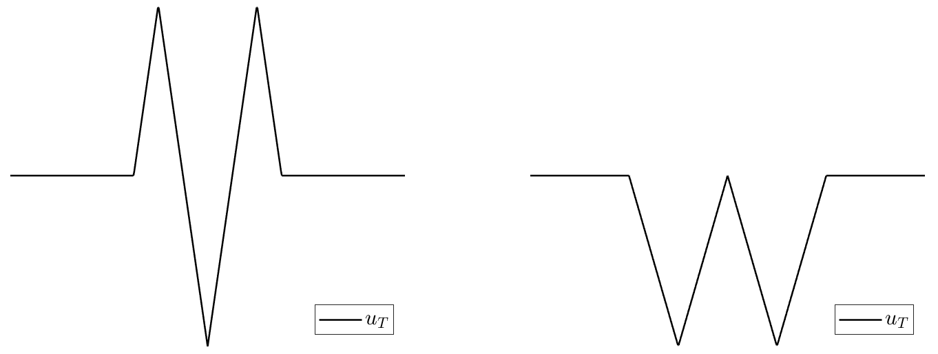 Figure 1: Two unreachable target functions in dimension 1.
We then start our study by characterizing the set of targets that are reachable.
In other words, for a given $u_T$ and $T>0$, we aim to determine whether or not there exists at least one initial condition $u_0$ satisfying $S_T^+ u_0=u_T$.
The natural candidate is the one obtained by reversing the time in the equation, considering $u_T$ as terminal condition. Here, we have to consider the class of backward viscosity solutions, for which the terminal-value problem associated to (HJ) is well-posed (see for example [1]).
We then define the backward operator as follows:
which associates to any terminal condition $u_T$, the function $w(0,\cdot)$,
i.e. the unique backward viscosity solution at time $0$, with terminal condition $u_T$.
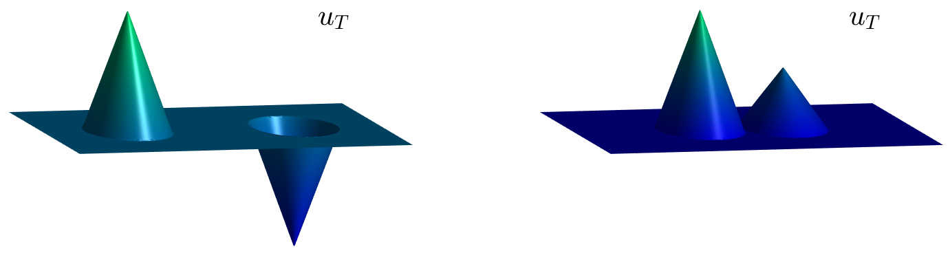 Figure 2: Two unreachable target functions in dimension 2.
Let us introduce, for a target $u_T$ and a time horizon $T>0$, the set
of initial conditions $u_0$ satisfying $S_T^+ u_0 = u_T$.
We say that a target $u_T$ is reachable for the time horizon $T$ if $I_T(u_T)\neq \emptyset$.
We can equivalently say that $u_T$ is an admissible observation at time $T>0$.
Here we give a result that identifies the set of reachable targets (or admissible observations) at time $T$,
with the fix-points of the composition operator $S_T^+\circ S_T^-$.
Theorem 1: Let $H$ satisfy (2), $u_T\in C^{0,1}(\mathbb{R}^n)$ and $T>0$. Then, the set $I_T(u_T)$ is nonempty
if and only if $S_T^+ \left( S_T^- u_T\right) = u_T.$
In other words, a target is reachable if and only if the initial condition $\tilde{u}_0:= S_T^- u_T$, obtained by applying the backward operator, satisfies $\tilde{u}_0\in I_T(u_T)$.
Or equivalently, an observation $u_T$ at time $T$ is admissible if and only if $S_T^+ \left( S_T^- u_T\right) = u_T.$
Projection on the set of reachable targets
In the case the observation $u_T$ at time $T$ is not admissible, maybe due to noise effects or to errors in the measurements, we can actually project it on the set of admissible observations by applying the operator $S_T^+\circ S_T^-$. For a given $u_T\in C^{0,1}(\mathbb{R}^n)$, we define this projection as follows:
Observe that $I_T(u_T^\ast)\neq \emptyset$ for any $u_T\in C^{0,1}(\mathbb{R}^n)$.
Indeed, $\tilde{u}_0:=S_T^- u_T\in I_T (u_T^\ast)$ by definition.
 Video 1: Projection of the examples in Figure 1 on the set of admissible observations at times $T=0.3$ and $T=0.8$ respectively.
In the Videos 1 and 2, we observe how the examples in Figures 1 and 2 are projected on the set of reachable targets.
We recall that the projection is obtained by solving the problem (HJ) backward in time and the forward.
Observe that, when the time goes backward, the solution is semiconvex, while in the forward resolution, it becomes semiconcave. See [1,4] for the classical results concerning this regularizing effect and [2] for the definition and properties of semiconcave and semiconvex functions.
 Video 2: Projection of the examples in Figure 2 on the set of admissible observations at time $T=1$.
Construction of initial data
Once we have projected the observation $u_T$ on the set of reachable targets at time $T$, we proceed to the construction of all the initial data $u_0$ satisfying $S_T^+ u_0 = u_T^\ast$.
This construction is contained in the recent work [3], and reads as follows:
Theorem 2: Let $H$ satisfy (2) and $T>0$.
Let $u_T\in C^{0,1}(\mathbb{R}^n)$ and define the functions
Then, for any $u_0\in C^{0,1} (\mathbb{R}^n)$, the two following statements are equivalent:
- $u_0\in I_T(u_T^\ast)$;
- $u_0(x)\geq \tilde{u}_0 (x), \ \forall x\in \mathbb{R}^n \quad \text{and} \quad u_0(x) = \tilde{u}_0(x), \ \forall x\in X_T(u_T^\ast),$
where $X_T(u_T^\ast)$ is the subset of $\mathbb{R}^n$ given by
In view of this result, we observe that, for a given admissible observation $u_T^\ast$ at time $T$,
the construction of the possible initial data can be carried out after obtaining the two following ingredients:
- the function $\tilde{u}_0 = S_T^- u_T^\ast$, obtained as the backward viscosity solution to (HJ) with terminal condition $u_T^\ast$;
- and the set $X_T(u_T^\ast)\subset \mathbb{R}^n$, that can be deduced from the differentiability points of $u_T^\ast$.
In Figures 3 and 4 below, we can see the scheme of the construction of all the initial data for the projection $u_T^\ast = S_T^+ (S_T^- u_T)$ of the non-admissible observations in Figure 1.
Observe that all the initial data in $I_T(u_T^\ast)$ must coincide with $\tilde{u}_0$ on the red region, while on the black region, they must be greater or equal than $\tilde{u}_0$.
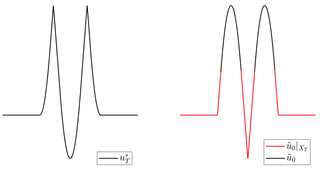 Figure 3: Reconstruction scheme for the admissible target obtained in Video 1 at the left.
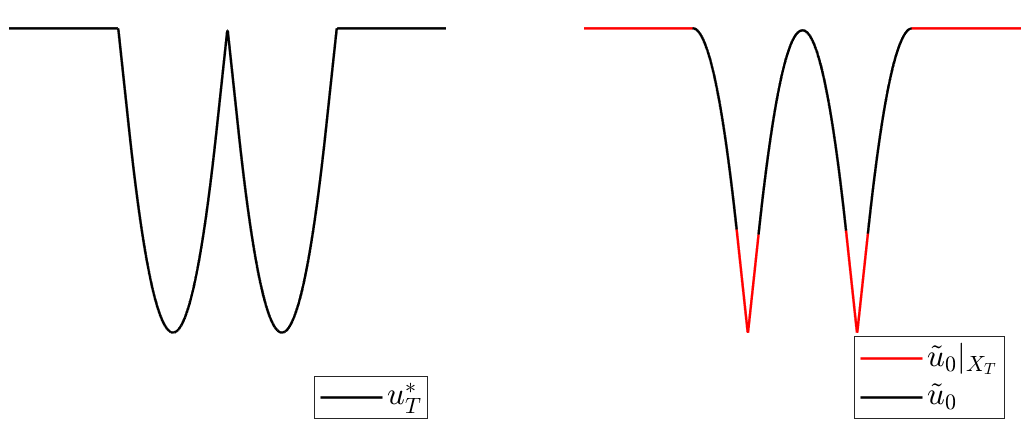 Figure 4: Reconstruction scheme for the admissible target obtained in Video 1 at the right.
An important consequence of Theorem 2 is that the initial data in $I_T(u_T^\ast)$ are not unique whenever $X_T(u_T^\ast) \neq \mathbb{R}^n$.
Indeed, the set $I_T(u_T^\ast)$ can be given in the following way:
In the case of the examples illustrated in Figures 3 and 4,
we can see in the videos 3 below, examples of different initial conditions whose solution coincides with $u_T^\ast$ at time $T$.
These exmaples have been generated randomly by adding to $\tilde{u}_0$ a nonegative a Lipschitz function vanishing in $X_T(u_T^\ast)$.
 Video 3: Examples of initial data $u_0\in I_T(u_T^\ast)$ for the reconstruction schemes depicted in Figures 3 and 4.
A possible interpretation of this reconstruction result is that the initial datum can only be reconstructed in the region $X_T(u_T^\ast)$, where it is uniquely determined by $\tilde{u}_0$,
while in the region $\mathbb{R}^n\setminus X_T(u_T^\ast)$, only a lower bound can be deduced.
In this last region, we can say that the information of the initial data has been partially lost after the time-interval $[0,T]$.
In the case of smooth solutions (when they exists) we have backward uniqueness, i.e. $I_T(u_T)$ is either empty or a singleton (see [1]).
In this case it holds that $X_T(u_T)=\mathbb{R}^n$.
Next, we see the reconstruction schemes for the examples depicted in Video 2, that correspond to the projection on the set of admissible observations of $u_T$ from Figure 2.
Observe the different structure of the set $\mathbb{R}^n\setminus X_T(u_T^\ast)$ (white region in the plot at the right)
in the surrounding area of bumps and wells of $u_T^\ast$.
- Near a bump, the set where $u_T^\ast$ is not differentiable is an isolated point, and then, it produces a ball for the set $\mathbb{R}^n\setminus X_T(u_T^\ast)$.
- Near a well, $u_T^\ast$ is non-differentiable on a circumference. This produces an annulus for the set $\mathbb{R}^n\setminus X_T(u_T^\ast)$.
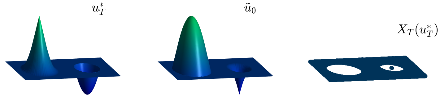 Figure 5: Reconstruction scheme for the admissible target obtained in Video 2 at the left.
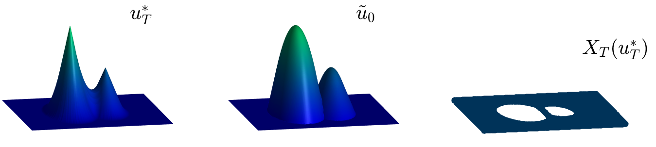 Figure 6: Reconstruction scheme for the admissible target obtained in Video 2 at the right.
Evolution of $X_T(u_T)$
As we have seen in the previous section, given an admissible observation $u_T$ of the solution at time $T$,
the initial datum can only be reconstructed in a region $X_T(u_T)$, while in its complementary, only a lower bound can be obtained.
Here, we are interested in the the role that $T$ plays in this reconstruction issue.
For this purpose, we fix an initial datum $u_0$ and then, for each $T>0$,
we construct the set $X_T(u_T)$, where $u_T := S_T^+ u_0$.
Our goal is to observe how $X_T(u_T)$ evolves as we increase $T$,
or in other words, we want to know what information from $u_0$ can be recoverd when the solution is observed at time $T$.
As we see in the following videos, $X_T(u_T)$ becomes smaller as we increase $T$, meaning that less information from the initial datum can be recovered if the observation is made after a long time interval.
In Figure 7 we fix two initial data in dimension 1.
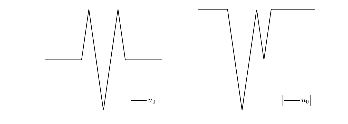 Figure 7: Two initial data in dimension 1.
Next, we can see in in Video 4, how the reconstruction scheme for $u_0$ (at the left in Figure 7) evolves as we increase the observation time.
For $T$ small, very little information is lost, however, for $T$ large, $X_T(u_T)$ only intersects the nonpositive region of $u_0$, and therefore, the two bumps can no longer be reconstructed.
 Video 4: Evolution of the target and the reconstruction scheme for the initial datum at the left in Figure 7.
In Video 5, we see the evolution of the reconstruction scheme for $u_0$ at the right in Figure 7.
In this case, $u_0$ is constituted of two wells, however, if the observation is made at time $T$ large enough, only the deepest well can be identified.
 Video 5: Evolution of the target and the reconstruction scheme for the initial datum at the right in Figure 7.
We end this blog post with three examples in the two-dimensional case.
Here we have the three examples of initial data that we have considered.
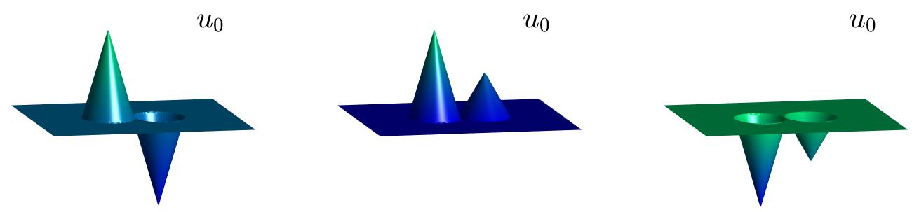 Figure 8: Three initial data in dimension 2.
In Video 6, we see the evolution of the reconstruction scheme for our first 2-dimensional example.
In this case, $u_0$ has a well and a bump. We observe that, as we increase the observation time $T$,
the white region, which corresponds to $\mathbb{R}^n\setminus X_T(u_T)$ becomes bigger and bigger.
This corresponds to the fact that, when the observation is made after a long time-interval, less information from the initial datum can be recovered. In addition, if we look at $u_T^\ast$ and $\tilde{u}_0$ in the two first plots, we see that the bump disappears for $T$ large enough.
This implies that after a long time-interval, the bump cannot be reconstructed.
 Video 6: Evolution of the reconstruction scheme for the first initial datum in Figure 8.
In Video 7, we see the evolution of the reconstruction scheme for the second example in Figure 8.
Here, the initial datum has two bumps of different height but same shape and size in their support.
Observe that, when $T$ is large enough, both bumps look the same, and therefore we cannot guess which one was taller at $t=0$. In fact, only the shape of their support can be reconstructed.
 Video 7: Evolution of the reconstruction scheme for the second initial datum in Figure 8.
In Video 8, we see the evolution of the reconstruction scheme for the third example in Figure 8.
Here, the initial datum has two wells of different depth.
We observe the same behaviour as in Video 5, where only the information of the deepest well is preserved for $T$ large enough.
 Video 8: Evolution of the reconstruction scheme for the third initial datum in Figure 8.
References
[1] E. Barron, P. Cannarsa, R. Jensen, C. Sinestrari, Regularity of Hamilton-Jacobi equations when forward is backward. Indiana University mathematics journal, pages 385-409, 1999.
[2] P. Cannarsa, C. Sinestrari, Semiconcave functions, Hamilton-Jacobi equations, and optmial control. volume 58. Springer Science & Business Media, 2004.
[3] C. Esteve, E. Zuazua, The inverse problem for Hamilton-Jacobi equations and semiconcave envelopes. Preprint <https://arxiv.org/abs/2003.06914
[4] P.L. Lions, Generalized solutions of Hamilton-Jacobi equations. volume 69. London Pitman, 1982.