Download Code
Burgers equation
For a given viscosity parameter $\nu$ and for time $t>0$, we consider the 2D Burgers equation on the unit square
with zero Neumann boundary conditions and initial condition
and its numerical approximation using
- Finite Elements in space and Runge-Kutta in time,
- a POD reduction of the FEM model, and
- a DMD reduced order model.
We present the basic ideas and how they are realized in a basic Python script.
0. The Setup
Please download and run the python file burgers.py to check the
implementation, to reproduce the presented results, and to the behavior of the
routines for different parameters.
Here is the start of the script that lists the modules on which the
implementation bases on.
import dolfin

import scipy.linalg as spla
import matplotlib.pyplot as plt
import numpy as np

from scipy.integrate import solve_ivp
from spacetime_galerkin_pod.ldfnp_ext_cholmod import SparseFactorMassmat
The code uses dolfin which is the python interface to
FEniCS while the other modules scipy, numpy,
and matplotlib are standard in python, I would say. The module
ldfnp_ext_cholmod is a little wrapper for the sparsity optimizing Cholesky
decomposition of sksparse.
It is available from my github
repository and falls back
to numpy routines, in the case that sksparse is not available.
1. The FEM Discretization
The spatial discretization in FEniCS
First, the mesh is defined – here a uniform triangulation of the unit square
controlled by the parameter N. For the value N=80 and for globally smooth
and piecewise quadratic ansatz functions, the resulting dimension of the system
is 51842.
# The mesh

pone = dolfin.Point(-1, -1)
ptwo = dolfin.Point(1, 1)
mesh = dolfin.RectangleMesh(pone, ptwo, N, N)

V = dolfin.VectorFunctionSpace(mesh, 'CG', 2)

### The FENICS FEM Discretization

v = dolfin.TestFunction(V)
u = dolfin.TrialFunction(V)
Next, the discrete linear operators are defined and exported as a SciPy sparse
matrix. Also, we factorize the mass matrix mmat for later use and define the
norm that is weighted with the mass matrix as this is the discrete $L^2$ norm.
# ## the mass matrix

mform = dolfin.inner(v, u)*dolfin.dx
massm = dolfin.assemble(mform)
mmat = dolfin.as_backend_type(massm).sparray()
mmat.eliminate_zeros()

# factorize it for later


mfac = SparseFactorMassmat(mmat)

# norm induced by the mass matrix == discrete L2-norm

def mnorm(uvec):
    return np.sqrt(np.inner(uvec, mmat.dot(uvec)))

# ## the stiffness matrix
# as a form in FEniCS

aform = nu*dolfin.inner(dolfin.grad(v), dolfin.grad(u))*dolfin.dx
aassm = dolfin.assemble(aform)

# as a sparse matrix

amat = dolfin.as_backend_type(aassm).sparray()
amat.eliminate_zeros()
Then we define the convective term as function of the velocity u both in terms
of an FE-function and as a function of the associated coefficient vector.
# ## the convective term

# as a function in FEniCS

def burgers_nonl_func(ufun):
    cform = dolfin.inner(dolfin.grad(ufun)*ufun, v)*dolfin.dx
    cass = dolfin.assemble(cform)
    return cass

# as a vector to form map

def burgers_nonl_vec(uvec):
    ufun = dolfin.Function(V)
    ufun.vector().set_local(uvec)
    bnlform = burgers_nonl_func(ufun)
    bnlvec = bnlform.get_local()
    return bnlvec
The Runge-Kutta Time Integration
To apply standard time integration schemes (here, RK23 turned out to be most
efficient), we define the right hand side $f_h$ of the spatially discretized problem
In this case the right hand side is an application of the discrete diffusion
and convection operator and the inverse of the mass matrix that, simply
speaking, maps a (discrete) form onto a discrete function. Note that there is no
explicit time dependency in the Burgers equation, but SciPy’s solve_ivp
requires this parameter. Also, we define the initial value here. The time grid
is used to store the solution for the snapshots needed later, but the time
integrator uses his internal time grid.
inivstrg = 'exp(-3.*(x[0]*x[0]+x[1]*x[1]))'
inivexpr = dolfin.Expression((inivstrg, inivstrg), degree=2)
inivfunc = dolfin.interpolate(inivexpr, V)
inivvec = inivfunc.vector().get_local()

burgsol = solve_ivp(brhs, (t0, tE), inivvec, t_eval=timegrid, method='RK23')
fullsol = burgsol.y
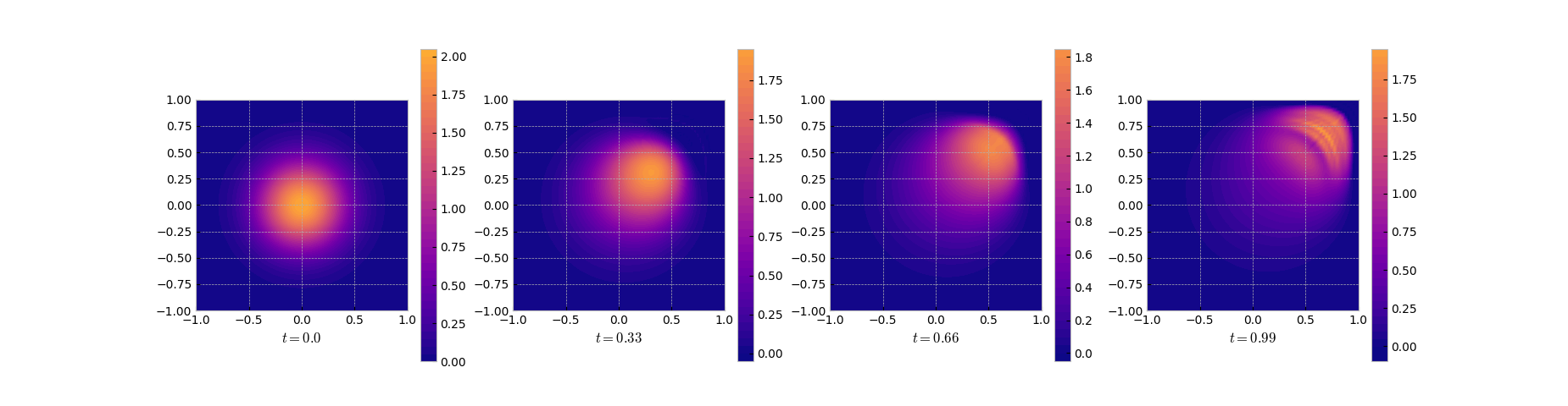
Here is the result. Note the sharp front that develops towards the end of the time
integration.
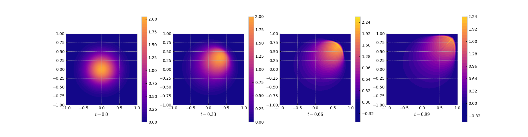
Solution snapshots of the full FEM model
2. POD Reduced Model
If one has snapshots of the solution $v _ h$ at some time instances $t _ i$ one
may well think that the span of the matrix of snapshots
is a good candidate for a space in which the solution evolves in. One may even
go further and look for a low-dimensional basis of this space. The span of a
matrix is best approximated by its dominant singular vectors. And this is the idea of
Proper Orthogonal Decomposition (POD) – use the leading singular vectors as a
basis for the solution space.
We use the Nts=101 snapshots of the FEM solutions to setup the matrix of
measurements $X$ and to compute the POD modes as $M^{-1/2}v _ k$, where $v _ k$
is the $k$-th leading left singular vector of $M^{1/2}X$. This procedure gives a
low-dimensional orthogonal (in the discrete $L^2$ inner product) basis that
optimally parametrizes the subspace of $L^2$ that is spanned by the solution
snapshots. In this example, we use the poddim=25 leading singular vectors
to define the reduced model.
snapshotmat = mfac.Ft.dot(burgsol.y)
podmodes, svals, _ = spla.svd(snapshotmat, full_matrices=False)
selected_podmodes = podmodes[:, :poddim]
podvecs = mfac.solve_Ft(selected_podmodes)
In this implementation we use a sparse factor of the mass matrix instead of the
square root. The singular values (in particular those that correspond to the
discarded directions) give an indication of how good the approximation is.
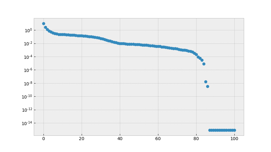
The singular values of the snapshot matrix
Here, the decay is comparatively slow, so that a one should not expect a good
low dimensional approximation by POD.
For the simulation, the state is parametrized by $u_h (t) \approx V \tilde
u_h(t)$ where $V$ is the matrix of the POD modes (in the code $V$ denoted by
podvecs), which gives a system in $\tilde u _ h$ with 25 degrees of freedom
(as opposed to the 51842 of the full order model).
redamat = podvecs.T.dot(amat.dot(podvecs))  # the projected stiffness

def redbrhs(time, redvec):
    inflatedv = podvecs.dot(redvec)
    redconv = podvecs.T.dot(burgers_nonl_vec(inflatedv))
    return -redamat.dot(redvec) - redconv.flatten()
Here we define the projected stiffness matrix and the reduced nonlinearity
through
- inflating the reduced state to full dimension
- applying the nonlinearity
- projecting down the result.
This means that our model is not completely independent of the full dimension.
For this problem there are hyperreduction techiques like DEIM.
Thus, the right hand side is readily defined the more that the projected mass
matrix is the identity. Why?
Finally, the initial value is projected into the reduced coordinates and the
reduced system is integrated in time.
redburgsol = solve_ivp(redbrhs, (t0, tE), prjinivvec,
                       t_eval=timegrid, method='RK23')
podredsol = redburgsol.y
In the solution we see that the reduced order model gives a decent approximation
in the smooth regime in the beginning and has its troubles approximating the front as can be seen in the error (log) plot.
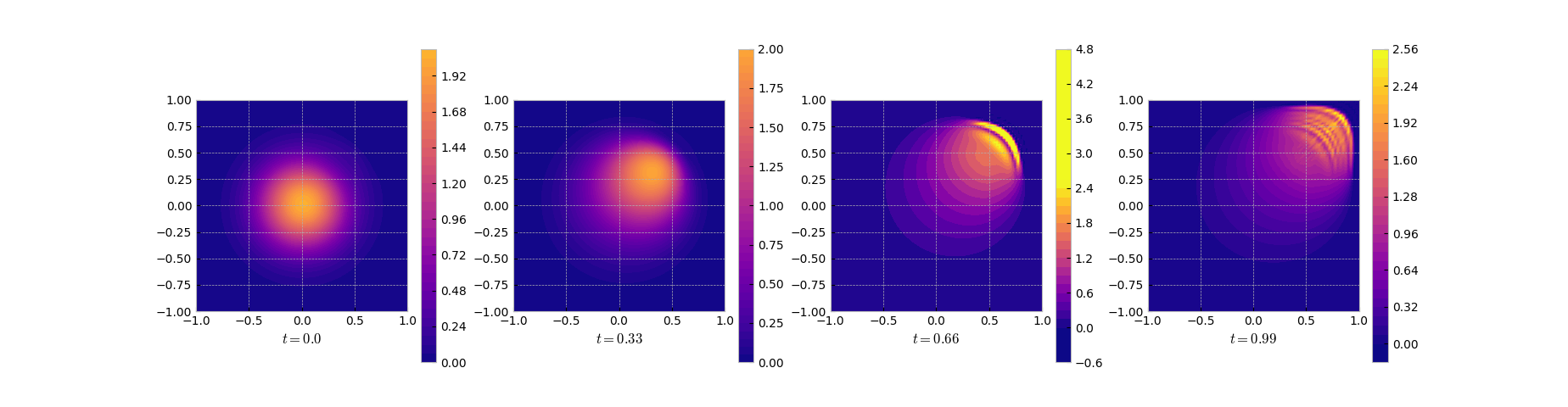
Snapshots of the solution of the reduced system
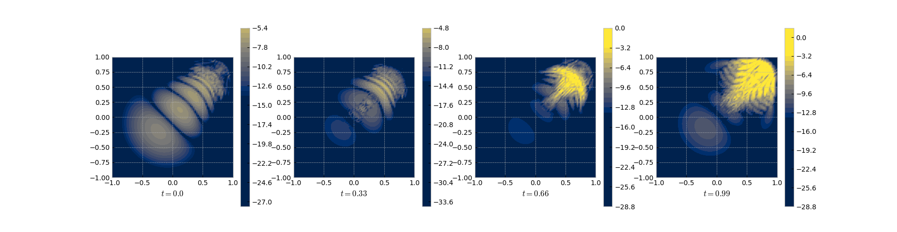
Snapshots of the log of the error between the full and the POD solution
3. DMD Reduced Model
POD is partially data driven – it uses data to create a basis but still
uses (a projection of) the model. If only snapshots but no model is given, one
may use the method of Dynamic Mode Decomposition (DMD) that tries to identify
a matrix $A$ that evolves the state like
In practice, one uses a set of snapshots and the two measurement matrices
and
Note that $X’$ is basically $X$ shifted by one time step.
Then the DMD matrix can be found by solving the linear regression problem
For the reduced DMD model we use the same snapshot matrix as for the POD. The
regression problem is solved via SVD to compute the needed pseudo inverse since
this naturally allows for a rank reduction and a factored representation of the
DMD matrix.
# ### dmd using truncated svd inverse

fburgsol = burgsol.y
Xmat = fburgsol[:, :-1]
Xdsh = fburgsol[:, 1:]
ux, sx, vxh = spla.svd(Xmat, full_matrices=False)
uxr, sxr, vxhr = ux[:, :poddim], sx[:poddim], vxh[:poddim, :]

# compute the dmd matrix in factored form: `dmda = dmdaone * dmdatwo`

dmdaone = Xdsh.dot(vxhr.T)
dmdatwo = np.linalg.solve(np.diag(sxr), uxr.T)
Once the DMD matrix $A$ is determined, the simulation of the DMD reduced model
is only a repeated multiplication by $A$.
# simulation of the dmd reduced model

dmdxo = inivvec
dmdsol = [dmdxo]
for k in np.arange(Nts):
    dmdsol.append(dmdaone.dot(dmdatwo.dot(dmdsol[-1])))

dmdsol = np.array(dmdsol).T
As can be seen from the results and the error plots, DMD does a good job in the
initial phase but fails in the region with the sharp front.
Snapshots of the DMD solution
It is commonly accepted that POD does not work well for transport dominated
problems – like the current case with the low viscosity parameter nu=1e-4.
So, I think that the results for POD are quite good noting that the reduced
order model has 25 degrees of freedom whereas the full model has 51842.
Nonetheless, in my tests, increasing the number of basis functions did not help
much. One can use a larger nu to get better POD approximations.
The DMD approach shows a similar performance. If compared to POD, the
qualitative approximation looks less good but the numbers are slightly better.
All in all, the DMD approximation seems less reliable as for some parameter
choices, the performance severely deteriorated.
Differential Equations.* arXiv:1611.04050
Decomposition: Theory and Applications* arXiv:1312.0041