The problem
We consider the following one-dimensional Burgers equation
where $u$ is the state, $u_0$ is the initial state and the flux function $f$ is defined by $f(u)=\frac{u^2}{2}$. Kruzkov’s theory provides existence and uniqueness of a solution of \eqref{eq} with initial datum $u_0 \in L^{\infty}(\mathbb R)$. This solution is called a weak-entropy solution, denoted by $(t,x) \to S_t^+(u_0)(x)$. For a given target function $u^T$, we introduce the backward entropy solution $(t,x) \to S^-_{t}(u^T)(x)$ as follows:
for every $t\in [0,T]$, for a.e $x\in \mathbb R$,
We study the problem of inverse design for \eqref{eq}. This problem consists in identifying the set of initial data evolving to a given target at a final time.
Due to the time-irreversibility of the Burgers equation, some target functions are unattainable from weak-entropy solutions of this equation, making the inverse problem under consideration ill-posed. To get around this issue, we introduce the following optimal control problem
where $u^T$ is a given target function and the class of admissible initial data $\mathcal{U}^0_{\text{ad}}$ in \eqref{opt2} is defined by
Above, stands for functions of bounded variation and $C>0$ is a constant large enough. The study of \eqref{opt2} is motivated by the minimization of the sonic boom effects generated by supersonic aircrafts [2].
To solve the optimal control problem \eqref{opt2}, some difficulties arise from a theoretical and numerical point of view.
- Since the entropy solution $u$ of \eqref{eq} may contain shocks even if the initial datum is a smooth function, this generates important added difficulties that have been the object of intensive study in the past, see [3,4] and the references therein. In particular, the authors make sense of the derivative of $J_0$ in \eqref{opt2} in a weak way by requiring strong conditions on the set of initial data. This leads to require that entropy solutions of \eqref{eq} have a finite number of non-interacting jumps.
- When $J_0$ is weakly differentiable, gradient descent methods have been implemented in [1,5,6] to solve numerically the optimal problem \eqref{opt2}. In the cases where it was applied successfully, only one possible initial datum emerges, namely the backward entropy solution $S_T^-(u^T)$. This is mainly due to the numerical viscosity that numerical schemes introduce to gain stability. To find some multiple minimizers, the authors in [8] use a filtering step in the backward adjoint solution.
Dans [9], we fully characterize the set of minimizers of the optimal control problem \eqref{opt2}.
Theorem 1. Let $u^T\in BV(\mathbb R)$. The optimal control problem \eqref{opt2} admits multiple optimal solutions. Moreover, for a.e $T>0$, the initial datum $u_0\in BV(\mathbb R)$ is an optimal solution of \eqref{opt2} if and only if $u_0 \in BV(\mathbb R)$ verifies $S_T^+(u_0)=S_T^+ (S_T^-(u^T))$.
A characterisation of the set is given in [7]. An illustration of Theorem 1. is given in Figure 1.
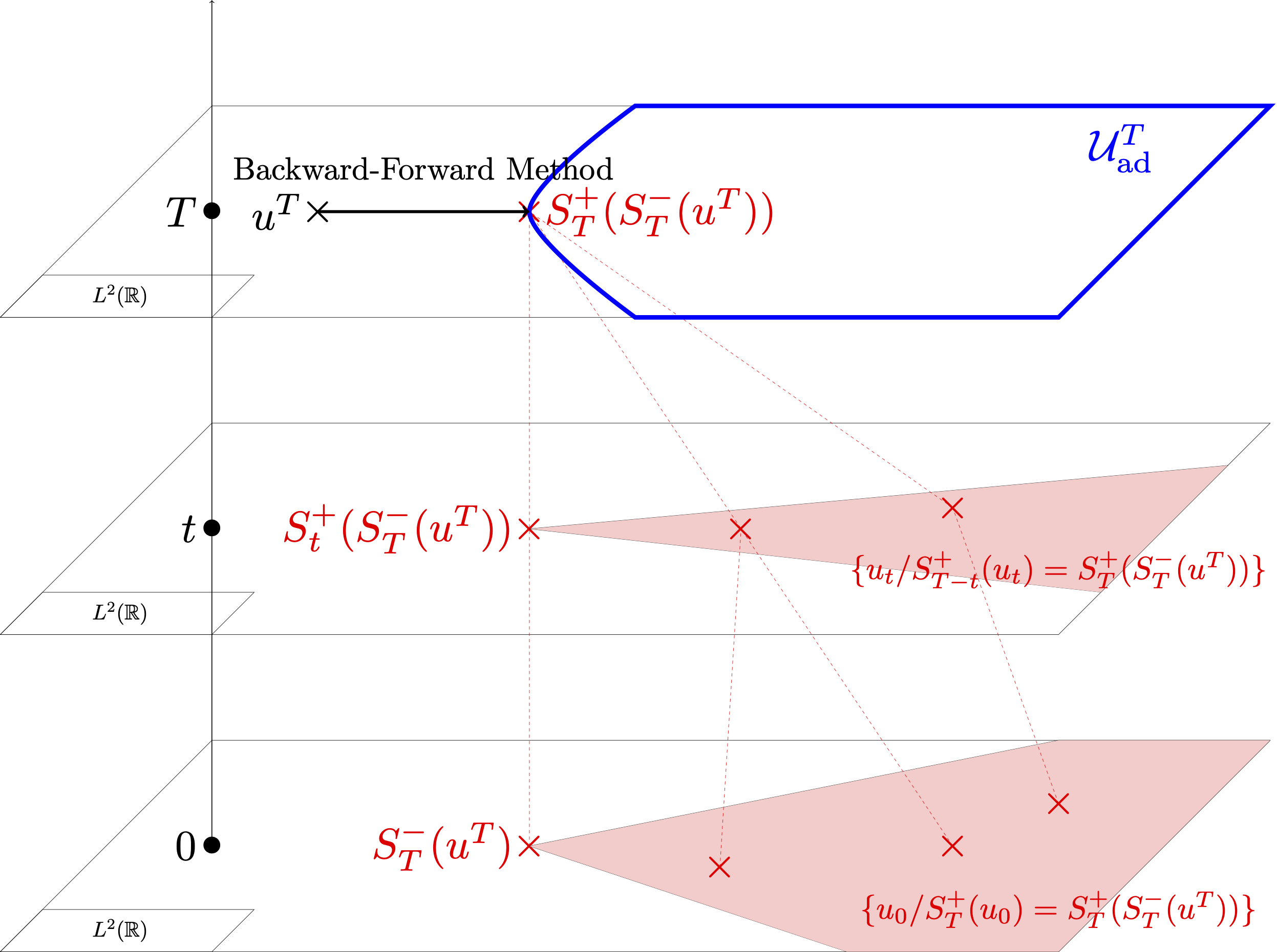
Figure 1: The backward-forward solution $S_T^+(S_T^-(u^T))$ is the projection of $u^T$ onto the set of attainable target functions. The shaded area in red at time $t=0$ represents the set of minimizers of \eqref{opt2}
The proof of Theorem 1 is structured as follows. From [7, Theorem 3.1, Corollary 3.2] or [8, Corollary 1], there exists $u_0\in BV(\mathbb R)$ such that if and only if satisfies the one-sided Lipschitz condition, i.e
Thus, the optimal problem \eqref{opt2} can be rewritten as follows.
where the admissible set $\mathcal{U}^T_{\text{ad}}$ is defined by
Above, $K_1$ an open bounded interval large enough. Note that the optimal problem \eqref{opt5} is not related to the PDE model \eqref{eq}. We prove that $q=S_T^+ (S_T^-(u^T))$ is a critical point of \eqref{opt5} using the first-order optimality conditions applied to \eqref{opt5} and the full characterization of the set given in [9, Theorem A.2].
Numerical simulations
In [9,Section 3], we implement a wave-front tracking algorithm to construct numerically the set of minimizers of \eqref{opt2}. We consider for instance, a target function defined by
From Theorem 1, the backward solution is an optimal solution of \eqref{opt2} and is an optimal solution of \eqref{opt2} if and only if . In Figure 2, the target function , the backward solution and the backward-forward solution are plotted.
|
|
|
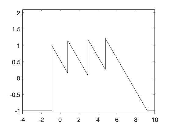
$x\to S^{-}_T(u^T)(x)$
|
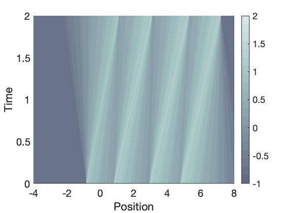
$(t,x)\to S^{+}_t(S^{-}_T(u^T))(x)$
|
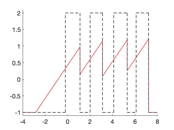
$u^T$ and $\color{red}{x\to S^{+}_T(S^{-}_T(u^T))(x)}$
$ $
Figure 2. Plotting of the target function $u^T$ defined in \eqref{uT}, the optimal solution $S_T^-(u^T)$ and the backward-forward solution $\color{red}{S^{+}_T(S^{-}_T(u^T))}$.
Note that has four different shocks located at $x=1.1$, $x=3.1$, $x=5.3$ and $x=7.2$. If we use a conservative numerical method as Godunov scheme, the approximate solution of doesn’t have shocks because of numerical viscosity that numerical schemes introduced, see Video 1.
Video 1. Approximate solution of $S_T^+(u_0)$ with $u_0$ an $N$-wave constructed with $ \color{red}{\text{a wave-front tracking algorithm}}$ and $\color{blue}{\text{a Godunov scheme}}$
This implies that only one minimizer of \eqref{opt2} can be constructed using a Godunov scheme, which is the backward entropy solution $S_T^-(u^T)$. When a wave-front tracking algorithm is implemented, the approximate solution of $S_T^+(S_T^-(u^T))$ has shocks since we track the possible discontinuities from $u^T$ to $S_T^+(S_T^-(u^T))$. This implies that all initial data $u_0$ that coincide with the approximate solution of $S_T^+ (S_T^-(u^T))$ can be recovered, see [9,Section 3].
In Video 2, we show that the weak-entropy solution of \eqref{eq} with initial data $S_T^-(u^T)$ coincides with $S_T^+ (S_T^-(u^T))$ at time $T$.
Video 2. Approximate solution of $(t,x) \to S_t^+(S_T^-(u^T))(x)$ using a wave-front tracking algorithm.
In Video 3, three other approximate optimal solutions $u_0$ of \eqref{opt2} are constructed. In particular, we show that $S_T^+ (u_0)=S_T^+ (S_T^-(u^T))$.
Video 3. Three approximate optimal solutions of \eqref{opt2} constructed using a wave-front tracking algorithm
[1] Navid Allahverdi, Alejandro Pozo and Enrique Zuazua. Numerical aspects of large-time optimal control of Burgers equation. ESAIM: Mathematical Modelling and Numerical Analysis, 50 (5):1371-1401,2016.
[2] Navid Allahverdi, Alejandro Pozo and Enrique Zuazua. Numerical aspects of sonic-boom minimization. A panorama of Mathematics: Pure and Applied, 658:267,2016.
[3] François Bouchut and François James. One-dimensional transport equations with discontinuous coefficients. Nonlinear Analysis, 32(7):891,1998.
[4] Alberto Bressan and Andrea Marson. A maximum principle for optimally controlled systems of conservation laws. Rendiconti del Seminario Matematico della Universita di Padova, 94:79-94, 1995.
[5] Carlos Castro, Francisco Palacios and Enrique Zuazua. An alternating descent method for the optimal control of the inviscid Burgers equation in the presence of shocks. Mathematical Models and Methods in Applied Sciences, 18(03):369-416,2008.
[6] Carlos Castro, Francisco Palacios and Enrique Zuazua. Optimal control and vanishing viscosity for the Burgers equation. In Integral Methods in Science and Engineering, Volume 2, pages 65-90. Springer, 2010.
[7] Rinaldo Colombo and Vincent Perrollaz. Initial data identification in conservation laws and Hamilton-Jacobi equations. arXiv preprint arXiv:1903.06448,2019.
[8] Laurent Gosse and Enrique Zuazua. Filtered gradient algorithms for inverse design problems of one-dimensional Burgers equation. In Innovative algorithm and analysis, pages 197-227. Springer, 2017.
[9] Thibault Liard and Enrique Zuazua. Inverse design for the one-dimensional Burgers equation. Submitted (2019).