1. Adjoint estimation: low or high order?
Adjoint methods have been systematically associated to the optimal control design [5] and their applications to aerodynamics [1, 4]. During the last decades, several works were oriented to develop a robust control theory based on the concepts of observability, optimality and controllability for linear and non-linear equations and systems of equations [2, 10, 11, 12].
Since the discrete approach forces to use the discrete adjoint problem of the flow solver to numerically solve the adjoint equation, the continuous approach is adopted due to its valuable flexibility of using different solvers for the flow and adjoint equations. It is well known that problems where high frequencies play an important role such as the control of wave equation [11]
The focus is put on the 2D linear scalar transport equation, that can be expressed in a conservative form as follows:
(1) 
where  is a time-independent velocity field of propagation.
Given a target function  , the aim in the 2D inverse design problem consists in finding
  such that
  via the minimization of a functional
  :
:
(2) 
This problem can be easily addressed by simply solving the transport equation backwards in time because of the time reversibility of the model. But such a simple approach fails as soon as the model involves nonlinearities (leading to shock discontinuities) or diffusive terms, making the system time-irreversible.
We are thus interested in the development of gradient descent methods with the aid of the adjoint equation (solved backwards in time) that can be easily deduced
(3) 
where  is the adjoint variable.
In order to achieve a good match with the continuous solutions, high order numerical schemes need to be used for the forward state equation (1). Here we shall use a second order scheme. Our main objective is to test the convenience of using the same order of accuracy when solving the adjoint equation or, by the contrary, to employ a low order one. When implementing the gradient descent iterations, the numerical scheme employed for solving the adjoint equation determines the direction of descent. Hence, different solvers for the adjoint system provide different results that can be compared in terms of accuracy and efficiency.
A gradient-adjoint iterative method is based on iterating a loop where the equation of state (flow equation) is solved in a forward sense while the adjoint equation, which is of hyperbolic nature as well, is solved backwards in time (see Figure 1).
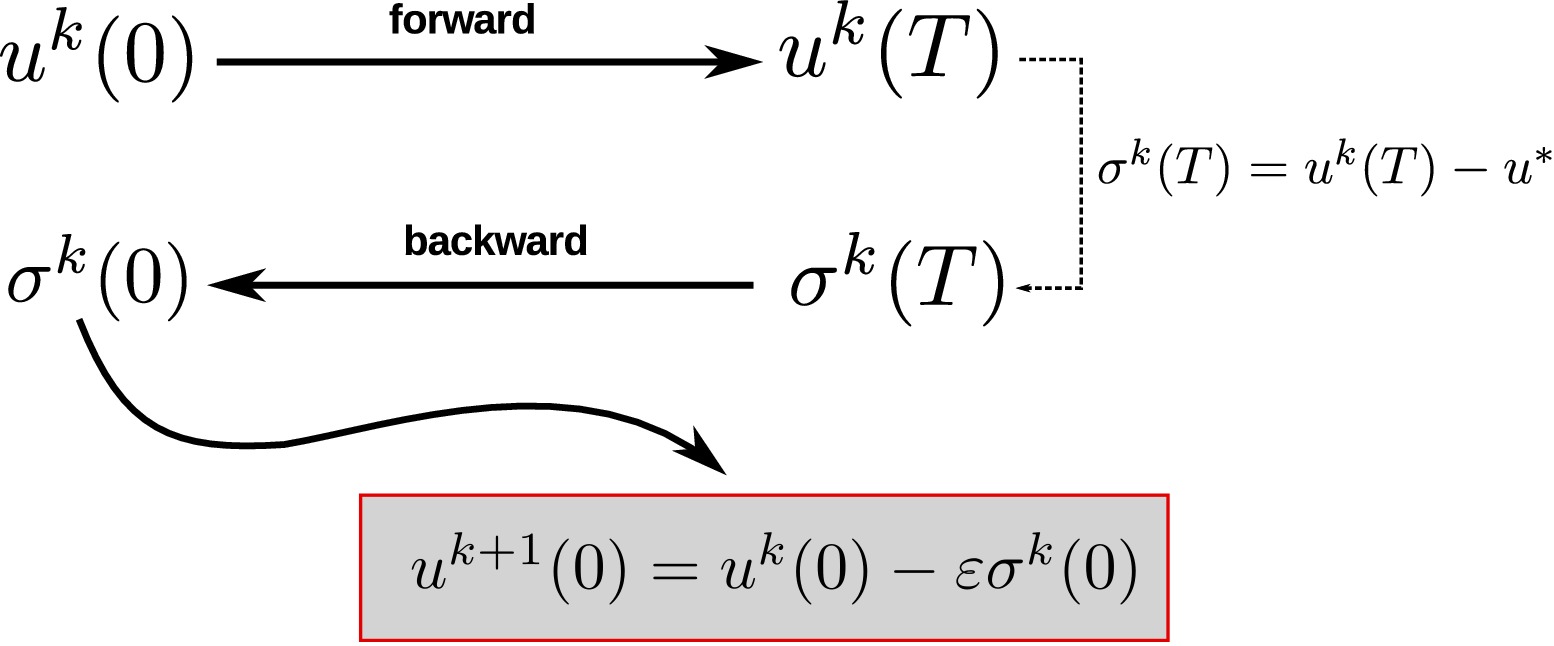 Figure 1. Iteration of the 2D inverse design
The adequate resolution of this loop is the main question addressed in this work, paying attention not only to accuracy but also to reducing its computational complexity. One could expect that the choice of high order numerical methods to solve both the equation of state and the adjoint one should provide the best results in terms of accuracy, at the prize of a high computational cost. But this is not always true and it is possible to relax the necessity of using the same order of accuracy for the resolution of the adjoint equation, not only reducing considerably the computational time needed by the complete loop but also achieving the same order of accuracy on the approximation of the inverse design, which is our ultimate goal.
2. 2D linear equation and continuous adjoint derivation
We focus on the following conservative linear transport scalar equation with an heterogeneous time-independent vector field 
(4) 
Obviously, the solution  exists and it is unique and can be determined by means of the method of characteristics provided
  is smooth enough (say,
  ). Thus, for all initial data
  there exists an unique solution in the class
 ![C([0, T]; L^2(\mathbb{R}^2))](https://cmc.deusto.eus/wp-content/ql-cache/quicklatex.com-de30d63fe67346256424d4f29592b08c_l3.png "Rendered by QuickLaTeX.com") .
.
Let us consider the inverse design problem: Given a target function  at
at  , to determine the initial condition such that
  .
.
The problem could be easily addressed solving the equation (4) backwards in time from the final datum  at , to determine
  exactly. But we are interested in addressing it from the point of view of optimal control. Let us therefore define the following functional, as a classical measure of the quadratic error with respect to the target function :
(5) 
The derivation of the adjoint equation can be achieved by simply multiplying by and integrating over a control volume ![\Omega \times [0,T]](https://cmc.deusto.eus/wp-content/ql-cache/quicklatex.com-2d4c316831b8619f3e16c795ef05083a_l3.png "Rendered by QuickLaTeX.com")
(6) 
Integrating by parts
(7) 
where  is the boundary and
  is the outward normal direction to the surface
  respectively.
It is feasible to take Gateaux derivatives with respect to the variable  in this identity getting:
(8) 
Gathering appropriately the terms:
(9) 
Let us select 
(10) 
and appropriate boundary conditions for  = 0. Hence (9) becomes
(11) ![\begin{equation*} \int_{\Omega} \left[\sigma (T) \delta u (T) - \sigma(0) \delta u(0)\right] dS = 0 \end{equation*}](https://cmc.deusto.eus/wp-content/ql-cache/quicklatex.com-9057b2491d4be9d4cc99b436123ccb5f_l3.png "Rendered by QuickLaTeX.com")
Assuming 
(12) 
On the other hand, it is also feasible to take the first variation of with respect to in (5)
(13) 
Finally,
(14) 
This derivation led to the adjoint equation  :
:
(15) 
 being the adjoint variable.
This equation measures the sensitivity of the solution to changes in the initial condition. It is worth mentioning that the adjoint equation is solved backwards in time (from to  ). In fact, system (15) is well-posed if and only if the original system is well posed in the forward sense.
3. Numerical schemes
In order to obtain a numerical solution based on a finite volume approach, (4) is integrated in a control volume ![\Omega_i \times [t^n,t^{n+1}]](https://cmc.deusto.eus/wp-content/ql-cache/quicklatex.com-e713a5583244ff2e528fd3d4199b2ae3_l3.png "Rendered by QuickLaTeX.com") where
where  represents each computational cell of the domain and
(16) 
Using the Gauss divergence theorem
(17) 
where  is the flux,
  denotes the surface surrounding the volume and
  its unit normal vector. The last contour integral in (17) can be replaced by the sum of the fluxes defined at each edge
  of length
  :
:
(18) 
with  is the number of edges of each cell
  (
( is for triangular grids) with neighbouring cells
  . Figure 2 clarifies the meaning of each variable.
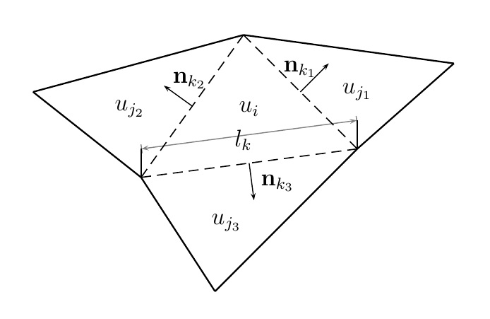 Figure 2. Sketch of the 2D finite volume approach
In this work two numerical schemes are proposed: a first order upwind (FOU) scheme and a second order upwind (SOU) scheme based on MUSCL-Hancock approach. The details of the implementation can be found in [7] and [6, 9] respectively. The use of a SOU scheme for the flow equation (forward) is mandatory in order to achieve the best accuracy since the FOU scheme is unable to capture the detail for the equation of state when trying to reach the target function. The issue of using one or another approach for solving the adjoint equation and, consequently, the gradient direction approach, is worth analysing.
4. Test case: Doswell frontogenesis
This test case was firstly proposed (in a forward sense) in [3]. It symbolizes the presence of horizontal temperature gradients and fronts in the context of meteorological dynamics. The original problem consists of a computational domain ![\Omega=[-5,5]](https://cmc.deusto.eus/wp-content/ql-cache/quicklatex.com-46ef7f79829f85449491de1fcd817e4b_l3.png "Rendered by QuickLaTeX.com") with open boundary conditions in which a front defined by the following initial condition:
with open boundary conditions in which a front defined by the following initial condition:
(19) 
is advected under the velocity field given by
(20) 
where  . The exact solution (the projection or restriction of the analytical solution on the computational mesh) on the whole space
  has the following explicit form:
(21) 
It is important to mention that the velocity field is divergence-free. The state equation can the be written similarly in divergence or non-divergence form:
(22) 
because
![\[\nabla \cdot \mathbf{v} \equiv 0,\]](https://cmc.deusto.eus/wp-content/ql-cache/quicklatex.com-49e362893033310594c5349ebaf6b112_l3.png "Rendered by QuickLaTeX.com")
This allows us to formulate the problem of inverse design. Given the exact value of the solution at time , i.e. giving (21) as a target function at , we aim to recover by a computational version of the gradient-adjoint methodology described above, an accurate and efficient approximation of the initial datum (19).
In our numerical experiments we take the values  and
and  . The exact initial condition and the exact target are shown in Figure 3 (left and right respectively). As can be seen, the target presents a vortex-type profile, due to the heterogeneous geometry of the velocity field.
Our goal is to build a numerical method capable of predicting accurately and efficiently an approximation of (19) out of the target (21) by means of a numerical version of the optimisation algorithm above.
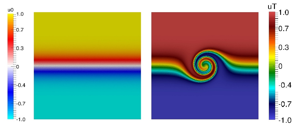 Figure 3: Doswell frontogenesis: Exact initial condition (left) and target function (right) for the inverse problem
The domain is discretized in 39998 unstructured triangles using Triangle [8] in a uniform Delaunay mesh. The initial condition for the first iteration is  . Both the forward and backward resolution are parallelized with OPENMP in 4 cores. The maximum number of iterations for the gradient method is set to 75, a constant step
  is selected and the Courant number is set to
  .
.
Additionally, the step size  is set as a constant at the beginning of each iteration. However, if the convergence is not guaranteed, i.e.,
  , the step size is halved until
  . Therefore, the stopping criteria for the iterative algorithm are:
- To reach the maximum number of iterations
- To achieve the maximum allowable error of the functional, in this case,

- To descend below
 when halving the step size trying to achieve convergence.
The numerical results are shown in Figures 4, 5 and 6 for the target  , initial condition
  and adjoint
  respectively at the last iteration of the gradient method. On the left side the
  approach is displayed while the
  resolution is illustrated on the right side.
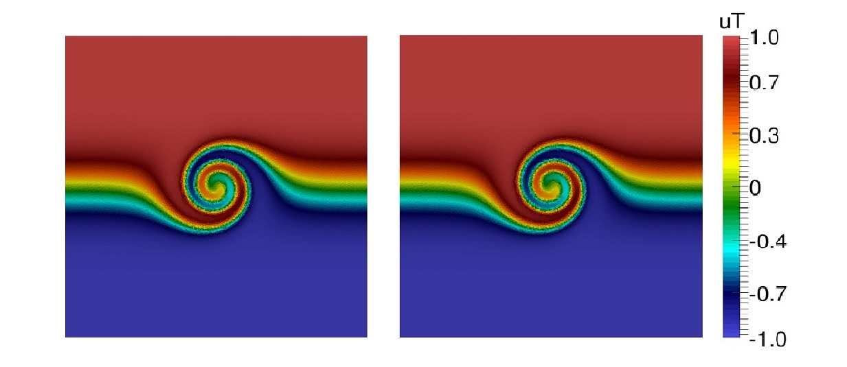 Figure 4: Doswell frontogenesis: Numerical target achieved by (left) and (right)
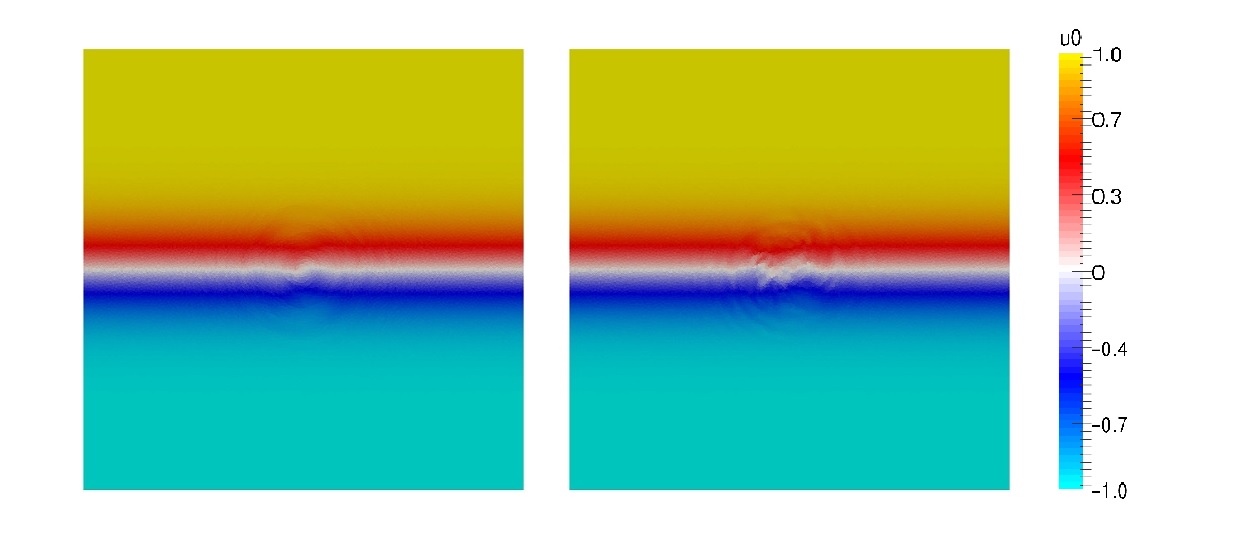 Figure 5: Doswell frontogenesis: Numerical initial condition achieved by (left) and (right)
In order to complete the qualitative results, the error computed as the difference between the exact and the numerical approximation is displayed in Figures 7 and 8 for the target  and the initial datum
  .
.
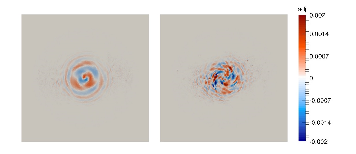 Figure 6: Doswell frontogenesis: Numerical adjoint variable
  achieved by (left) and (right)
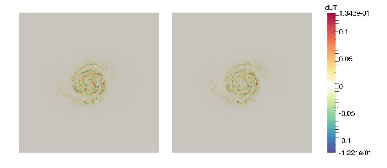 Figure 7: Doswell frontogenesis: Target error achieved by (left) and (right)
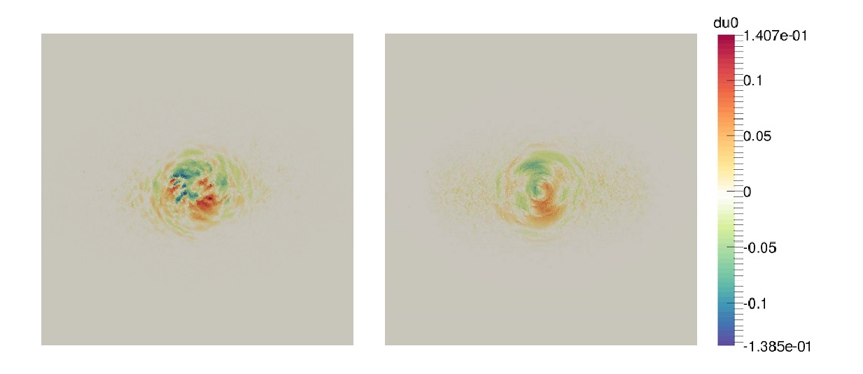 Figure 8: Doswell frontogenesis: Initial datum error achieved by (left) and (right)
Quantitative results can be obtained by means of the computation of  and
and  norms, not only with respect to the target function but also to the known exact initial condition
  in order to evaluate the results achieved by and :
(23) 
Table 1 condenses this information as well as the number of iterations and the CPU time for each proposed scheme. For the sake of clarity and for each comparison, the best results are highlighted in bold font.
| Scheme |
( ) ) |
 () () |
( ) ) |
() |
nIters |
CPU Time (s) |
|
FOU
|
1.37127e+00 |
1.37078e-01 |
1.36043e+00 |
8.64870e-02 |
75 |
366.26 |
|
SOU
|
1.23889e+00 |
1.34271e-01 |
1.88749e+00 |
1.40718e-01 |
45 |
488.61 |