Conservation laws in the presence of shocks

The problem

We analyze a model tracking problem for a 1D scalar conservation law. It consists in optimizing the initial datum so to minimize a weighted distance to a given target during a given finite time horizon. To be more precise, given a finite time $T > 0$, a target function $u^d\in L^2(\mathbb R\times(0,T))$, and a positive weight function $\rho\in L^\infty(\mathbb R\times(0,T))$ with compact support in $\mathbb R\times(0,T)$, we consider the functional cost to be minimized $J$, over a suitable class of initial data $\mathcal{U}_{ad}$, defined by

$$\begin{equation}\label{FunctionalJ} J(u^0)=\frac 1 2\int_0^T\int_{\mathbb{R}}\rho(x,t)|u(x,t)-u^d(x,t)|^2dxdt, \end{equation}$$

where $u:\mathbb R_x\times\mathbb R_t\to \mathbb R$ is the unique entropy solution of the scalar conservation law

$$\begin{equation}\label{conservativeEquation} \partial_t u+\partial_x(f(u))=0,\; \textrm{in }\mathbb R \times(0,T); \;\;\; u(x,0)=u^0(x),\; x\in\mathbb R. \end{equation}$$

Thus, the problem under consideration reads: To find $u^{0,min}\in\mathcal{U}_{ad}$ such that

$$\begin{equation}\label{optimalProblem} J(u^{0,min})=\min_{u^0\in\mathcal{U}_{ab}}J(u^0). \end{equation}$$

Here the flux $f:\mathbb R\to\mathbb R$ is assumed to be smooth: $f\in C^1(\mathbb R,\mathbb R)$. The initial datum $u^0$ will be assumed to belong to a suitable admissible class $\mathcal{U}_{ad}$ to ensure the existence of a minimizer.

Sensitivity of the state in the presence of shocks

Inspired in several results on the sensitivity of solutions of conservation laws in the presence of shocks in one-dimension (see [7, 4, 5, 6, 17, 13]), we focus on the particular case of solutions having a single shock. But the analysis can be extended to consider more general one-dimensional systems of conservation laws with a finite number of noninteracting shocks. We introduce the following hypothesis:

Hypothesis 1.1: Assume that $u(x,t)$ is a weak entropy solution of (\ref{conservativeEquation}) with a discontinuity along a regular curve $\Sigma={(\varphi(t),t),\;t\in(0,T)}$, which is Lipschitz continuous outside $\Sigma$. In particular, it satisfies the Rankine-Hugoniot condition on $\Sigma$

$$\varphi'(t)[u]_{\Sigma^t}=[f(u)]_{\Sigma^t}.$$

Here we have used the notation:

$$[v]_{\Sigma^t}=\lim\limits_{\varepsilon\searrow 0}v(\varphi(t)+\varepsilon,t) -v(\varphi(t)-\varepsilon,t)$$

for the jump at $\Sigma^t=(\varphi(t),t)$ of any piecewise continuous function $v$ with a discontinuity at $\Sigma^t$.

Note that $\Sigma$ divides $\mathbb R \times (0, T )$ into two parts: $Q_-$ and $Q_+$ , the sub-domains of $\mathbb R \times (0, T)$ to the left and to the right of $\Sigma$ respectively. As we will see, in the presence of shocks, to deal correctly with optimal control and design problems, the state of the system needs to be viewed as constituted by the pair $(u,\varphi)$ combining the solution of (\ref{conservativeEquation}) and the shock location $\varphi$. This is relevant in the analysis of sensitivity of functions below and when applying descent algorithms. We adopt the functional framework based on the generalized tangent vectors (see [7] and Definition 4.1 in [8]). Let $u^0$ be the initial datum, that we assume to be Lipschitz continuous to both sides of a single discontinuity located at $x = \varphi^0$, and consider a generalized tangent vector $(\delta u^0,\delta \varphi^0) \in L^1(\mathbb R) \times \mathbb R$ for all $0 \leq T$. Let $u^{0,\varepsilon}$ be a path which generates $(\delta u^0,\delta \varphi^0)$. For $\varepsilon$ sufficiently small, the solution $u^\varepsilon(\cdot,t)$ of (\ref{conservativeEquation}) is Lipschitz continuous with a single discontinuity at $x = \varphi^{\varepsilon}(t)$, for all $t \in [0,T]$. Therefore, $u^{\varepsilon}(\cdot, t)$ generates a generalized tangent vector $(\delta u(, t), \delta\varphi(t)) \in L^1(\mathbb R) \times \mathbb R$. Moreover, in [8] it is proved that it satisfies the following linearized system:

$$\begin{eqnarray} \label{1DlinearizedSystem01} \partial_t \delta u+\partial_x(f'(u)\delta u)&=&0,\;\;\;\;\;\;\;\;\;\;\;\;\;\;\;\;\;\;\;\;\;\;\;\;\;\;\;\;\;\;\;\;\;\;\;\;\text{in } Q_-\cup Q_+\\ \label{1DlinearizedSystem03} \frac{d}{dt}\left([u]_{\Sigma^t}\delta\varphi\right)&=&[f'(u)\delta u]_{\Sigma^t}-[\delta u]_{\Sigma^t}\frac{d}{dt}\varphi,\;\; t\in(0,T)\\ \label{1DlinearizedSystem02} \delta u(x,0)&=&\delta u^0(x),\;\;\;\;\;\;\;\;\;\;\;\;\;\;\;\;\;\;\;\;\;\;\;\;\;\;\;\{x<\varphi^0\}\cup\{x>\varphi^0\}\\ \label{1DlinearizedSystem04} \delta\varphi(0)&=&\delta\varphi^0. \end{eqnarray}$$

Sensitivity of the cost in the presence of shocks

In this section we study the sensitivity of the functional $J$ with respect to variations associated with the generalized tangent vectors defined in the previous section. We first define an appropriate generalization of the Gateaux derivative of $J$.

Definition 1.2: Let $J : L^1(\mathbb R) \to \mathbb R$ be a functional and $u^0 \in L^1(\mathbb R)$ be Lipschitz continuous with a discontinuity in $\Sigma^0$, an initial datum for which the solution of (\ref{conservativeEquation}) satisfies hypothesis (1.1). $J$ is Gateaux differentiable at $u^0$ in a generalized sense if for any generalized tangent vector $(\delta u^0,\delta \varphi^0)$ and any family $u^{0,\varepsilon}$ associated to $(\delta u^0, \delta \varphi^0)$ the following limit exists,

$$\delta J=\lim_{\varepsilon\to 0}\frac{J(u^{0,\varepsilon})-J(u^0)}{\varepsilon},$$

and it depends only on $(u^0,\varphi^0)$ and $(\delta u^0,\delta\varphi^0)$, i.e. it does not depend on the particular family $u^{0,\varepsilon}$ which generates $(\delta u^0,\delta\varphi^0)$. The limit is the generalized Gateux derivative of $J$ in the direction $(\delta u^0,\delta\varphi^0)$. </i>

The following result easily provides a characterization of the generalized Gateaux derivative of $J$ in terms of the solution of the associated adjoint system (\ref{1DSystemAdj}).

Proposition 1.3: The Gateaux derivative of $J$ can be written as follows

$$\begin{equation} \label{GateauxDerivativeJ02} \delta J(u^0)[\delta u^0,\delta\varphi^0]=\int_{\RR}p(x,0)\delta u^0(x) dx-q(0)[u]_{\Sigma^0}\delta\varphi^0, \end{equation}$$

where the adjoint state pair $(p,q)$ satisfies the system

$$\begin{eqnarray} \label{1DSystemAdj} -\partial_t p-f'(u)\partial_x p&=&\rho\,(u-u^d),\;\;\;\;\;\;\;\;\;\;\;\;\;\;\;\;\;\;\;\;\;\;\;\;\;\;\;\;\;\;\;\;\;\;\;\; \text{in } Q_-\cup Q_+\\ \,[p]_{\Sigma^t}&=&0,\;\;\;\;\;\;\;\;\;\;\;\;\;\;\;\;\;\;\;\;\;\;\;\;\;\;\;\;\;\;\;\;\;\;\;\;\;\;\;\;\;\;\;\;\;\;\;\;\; t\in(0,T) \label{1Dadjoint0202}\\ q(t)&=&p(\varphi(t),t),\;\;\;\;\;\;\;\;\;\;\;\;\;\;\;\;\;\;\;\;\;\;\;\;\;\;\;\;\;\;\;\;\;\;\;\;\; t\in (0,T)\label{1Dadjoint0203}\\ -\frac{d}{dt}q&=&\frac{(1+(\dot{\varphi})^2)^{1/2}[\rho\,(u-u^d)^2]_{\Sigma^t}}{2[u]_{\Sigma^t}},\;\;\;\;\;\;\;\;\; t\in (0,T) \label{1Dadjoint03} \\ p(x,T)&=&0,\;\;\;\;\;\;\;\;\;\;\;\;\;\;\;\;\;\;\;\;\;\;\;\;\;\;\;\;\;\;\;\;\;\;\;\;\;\;\;\{x<\varphi(T)\}\cup\{x>\varphi(T)\} \label{1Dadjoint02}\\ q(T)&=&0. \label{1Dadjoint04} \end{eqnarray}$$

Let us briefly comment the result of Proposition 1.3 before giving its proof. System (\ref{1DSystemAdj}) has a unique solution. In fact, to solve the backward system (\ref{1DSystemAdj}) we first define the solution $q$ on the shock $\Sigma$ from the conditions for $q$. This determines the value of $p$ along the shock. We then propagate this information to both sides of $\Sigma$, by characteristics (see Figure 1 where we illustrate this construction).

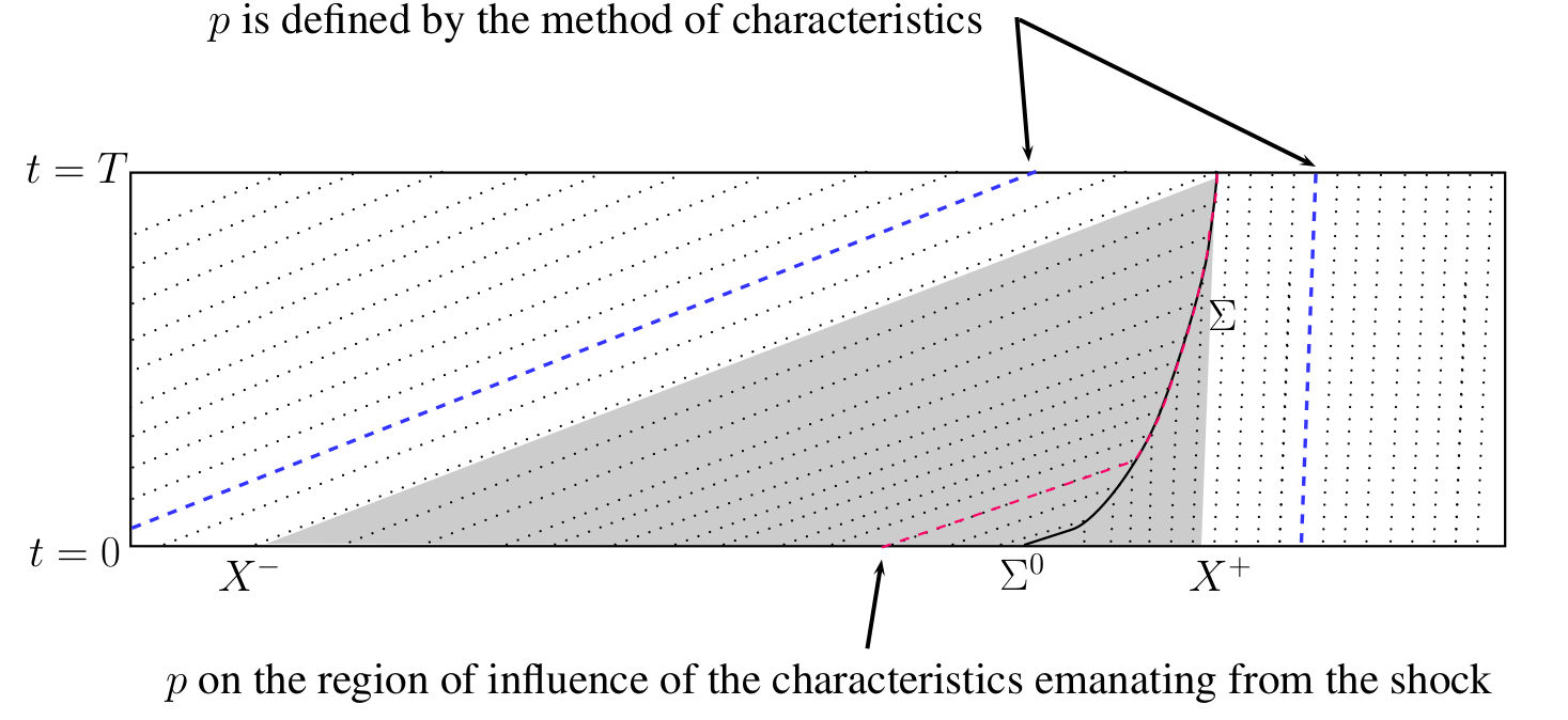Figure 1: Characteristic lines entering on a shock and how they may be used to build the solution of the adjoint system both away from the shock and on its region of influence.

Formula (\ref{GateauxDerivativeJ02}) provides an obvious way to compute a first descent direction of $J$ at $u^0$. We just take

$$\begin{equation}\label{descentDirection01} (\delta u^0,\delta \varphi^0)=(-p(\cdot,0),q(0)[u]_{\Sigma^0}). \end{equation}$$

Here, the value of $\delta \varphi^0$ must be interpreted as the optimal infinitesimal displacement of the discontinuity of $u^0$.

In [8], when considering the inverse design problem, it was observed that the solution $p$ of the corresponding adjoint system at $t=0$ was discontinuous, with two discontinuities, one in each side of the original location of the discontinuity at $\Sigma^0$. This was a reason not to use this descent direction and for introducing the alternating descent method. In the present setting, however, the adjoint state $p$ obtained is typically continuous. This is due to the fact that $p$ at both side of the discontinuity is defined by the method of characteristics and that, on the region of influence of the characteristics emanating from the shock, the continuity is preserved by the fact that, on one hand, $q=q(t)$ itself is continuous as the primitive of an integrable function and that the data for $p$ and $q$ at $t=T$ are continuous too. Despite of this, as we shall see, the implementation of the alternating descent direction method is worth since it significantly improves the results obtained by the purely discrete approach.

Numerical Experiments

In this section we present some numerical experiments which illustrate the results obtained in an optimization model problem with each one of the numerical methods described in the previous section. We have chosen as computational domain the interval $(-4, 4)$ and we have taken as boundary conditions in the numerical scheme, at each time step $t = t^n$, the value of the initial data at the boundary. This can be justified if we assume that the initial datum $u^0$ is constant in a sufficiently large inner neighborhood of the boundary $x = \pm 4$ (which depends on the size of the $L^\infty$-norm of the data under consideration and the time horizon $T$), due to the finite speed of propagation. A similar procedure is employed for the adjoint equation. We underline once more that the solutions obtained with each method may correspond to global minima or local ones since the gradient algorithm does not distinguish them. In the experiments we consider the Burgers’ equation, i.e. $f(z)=z^2/2$,

$$\begin{equation}\label{BurgerNumerica} \partial_tu+\partial_x\left(\frac{u^2}{2}\right)=0,\;\;\; u(x,0)=u^0(x). \end{equation}$$

The weight function $\rho$, under consideration in the experiments is given by

$$\rho(x,t)=\left\{ \begin{array}{cl} 1 & t\in ( T/2,T)\\ 0 & \text{otherwise.} \end{array} \right.$$

And the time horizon $T=1$. To compare the efficiency of the different methods we consider a fixed $\Delta x = 1/20, \lambda = \Delta t /\Delta x = 2/3$ (which satisfies the CFL condition). We then analyze the number of iterations that each method needs to attain a prescribed value of the functional.

Experiment 1

We first consider a piecewise constant target profile $u^d$ given by the solution of \ref{BurgerNumerica} with the initial condition $(u^d)^0$ given by

$$\begin{equation}\label{E1u0minimoa} (u^d)^0(x)=\left\{ \begin{array}{cl} 0.7 & x\in[-2,1]\\ 0 & \text{otherwise.} \end{array} \right. \end{equation}$$

Note that, in this case, \ref{E1u0minimoa} yields a particular solution of the optimization problem and the minimum value of $J$ vanishes. We solve the optimization problem \ref{optimalProblem} with the above described different methods starting from the following initialization for $u^0$:

$$\begin{equation}\label{Ep1u^0} u^0(x)=\left\{ \begin{array}{cl} 0.5 & x\leq 0\\ -0.1 & x>0, \end{array} \right. \end{equation}$$

which also has a discontinuity but located on a different point.

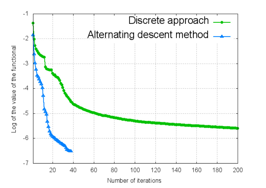Figure 2: Experiment 1. $\log (J)$ versus the number of iterations in the descent algorithm for the discrete and the alternating descent methods.

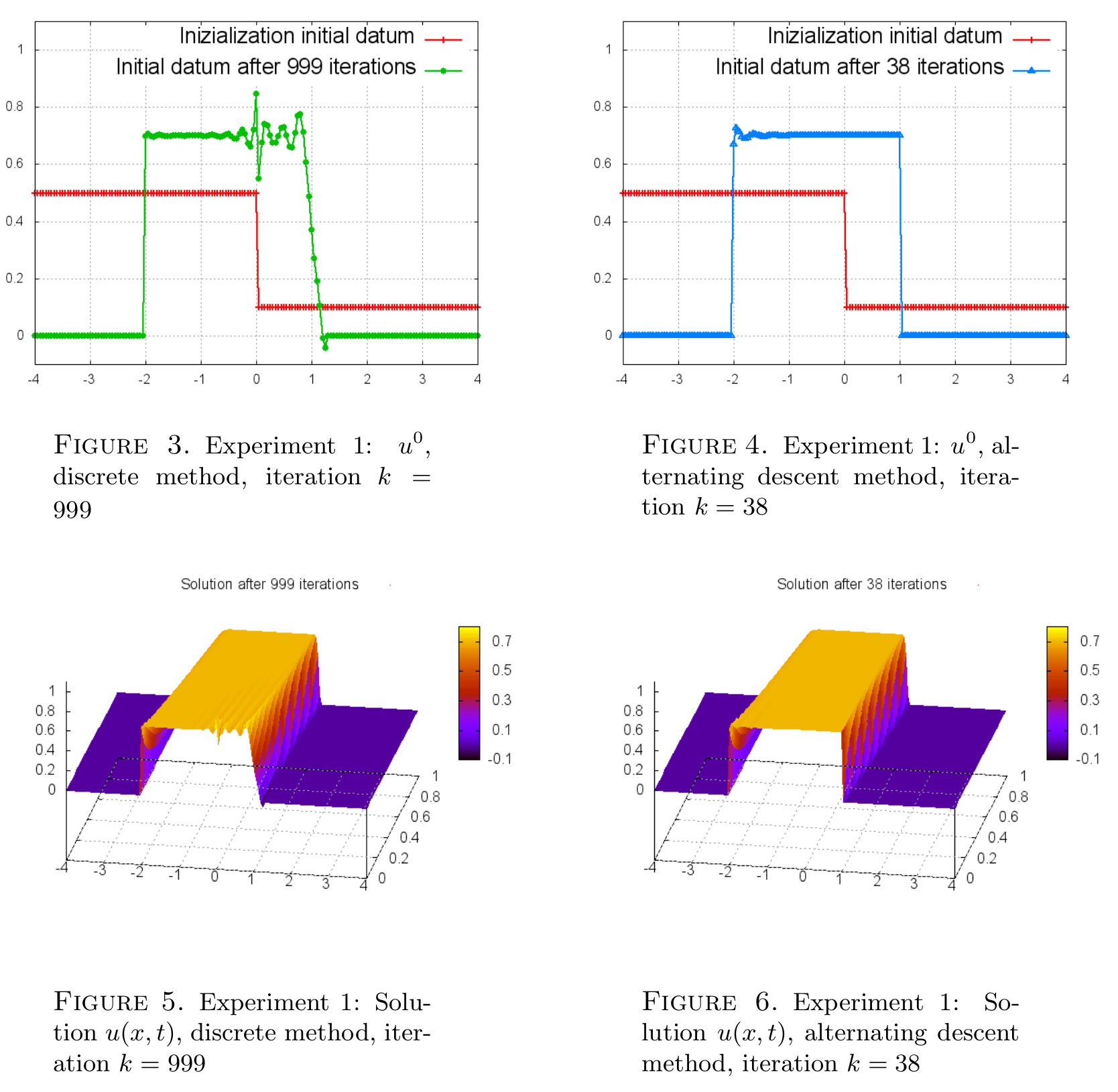
In Figures 3 and 4, we present the minimizers obtained by the methods above, and the associated solutions, Figures 5 and 6. The initial datum $u^0$ obtained by the alternating descent method (Figures 4) is a good approximation of \ref{E1u0minimoa}. The solution given by the discrete approach (Figure 3) presents added spurious oscillations. Furthermore, the discrete method is much slower and does not achieve the same level of accuracy since the functional $J_\Delta$ does not decrease so much.

 

Experiment 2

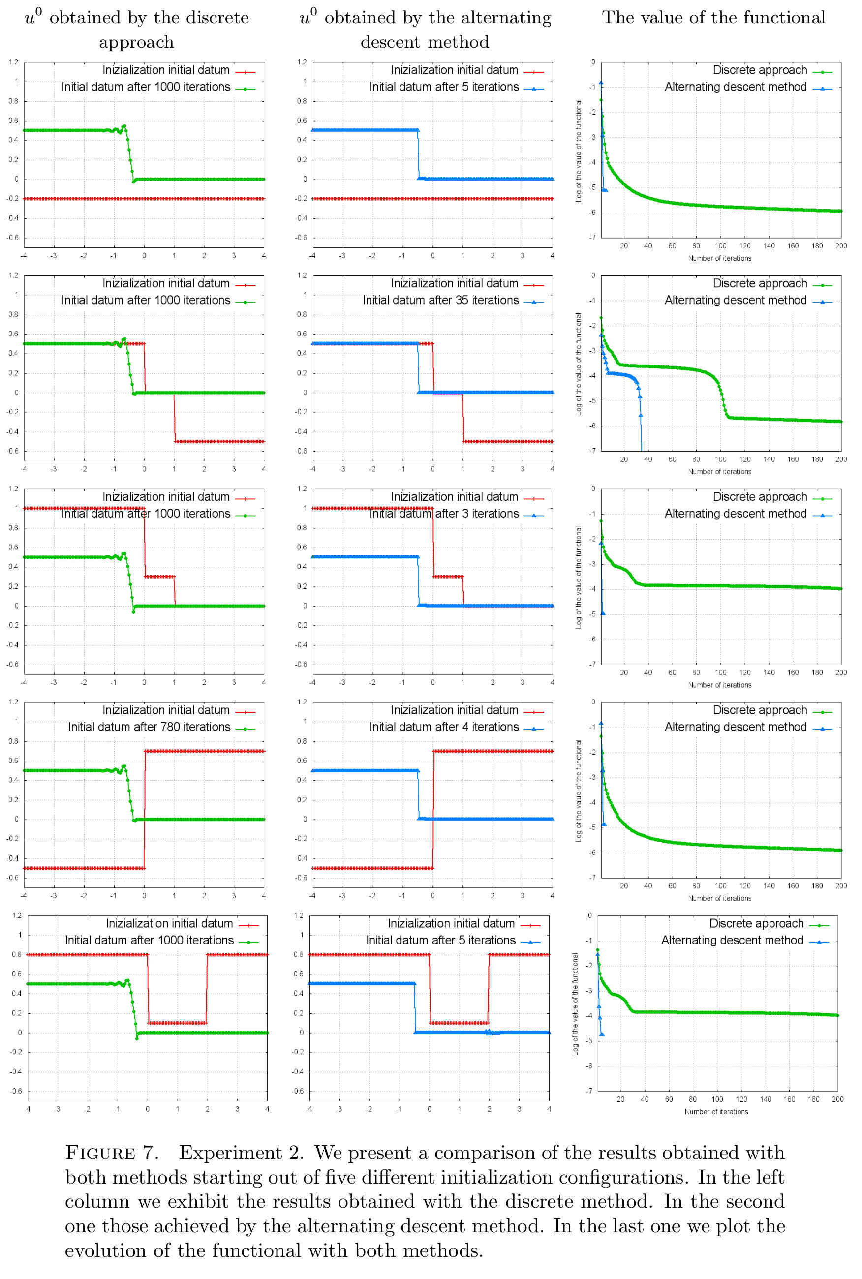
The previous experiment indicates that the alternating descent method performs significantly better. In order to show that this is a systematic fact, which arises independently of the initialization of the method, we consider the target $u^d$ given by the solution of \ref{BurgerNumerica} with the initial condition $(u^d)^0$ given by

$$\begin{equation}\label{E2u0minimo} (u^d)^0(x)=\left\{ \begin{array}{cl} 0.5 & x\leq 0.5\\ 0 & \text{otherwise,} \end{array} \right. \end{equation}$$

but this time we compare the performance of both methods starting from different initializations. The obtained numerical results are presented in Figure 7. We see that, regardless the initialization considered, the alternating descent method performs significantly better. We observe that in the five experiments the alternating descent method perfumes better ensuring the descent of the functional in much fewer iterations and yielding smoother, less oscillatory approximation of the minimizer. Note also that the discrete method, rather than yielding discontinuous approximations of the minimizer as the alternating descent method does, it produces an initial datum with a Lipschitz front. Observe that these are two different configurations that can lead to the same evolution for the Burgers equation after some time, once the front develops the discontinuity. This is in agreement with the fact that the functional to be minimized is only active in the time-interval $T/2 \le t \le T$.

 

Bibliography

[1] A. Adimurthi, S.S. Ghoshal and V. Gowda Optimal controllability for scalar conservation laws with convex flux. 12, Jan. 2012.

[2] D. Auroux and J. Blum Back and forth nudging algorithm for data assimilation problems. Comptes Rendus Mathematique, 340(12):873 – 878, 2005.

[3] D. Auroux and M. Nodet The back and forth nudging algorithm for data assimilation problems: theoretical results on transport equations. ESAIM: Control, Optimisation and Calculus of Variations, 18(2):318–342, 7 2012.

[4] C. Bardos and O. Pironneau A formalism for the differentiation of conservation laws. C. R. Math. Acad. Sci. Paris, 335(10):839–845, 2002.

[5] F. Bouchut and F. James One-dimensional transport equations with discontinuous coefficients. Nonlinear Anal., 32(7):891–933, 1998.

[6] F. Bouchut and F. James Differentiability with respect to initial data for a scalar conservation law. In Hyperbolic problems: theory, numerics, applications, Vol. I (Zürich, 1998), volume 129 of Internat. Ser. Numer.Math., pages 113–118. Birkhäuser, Basel, 1999.

[7] A. Bressan and A. Marson A variational calculus for discontinuous solutions of systems of conservation laws. Comm. Partial Differential Equations, 20(9-10):1491–1552, 1995.

[8] C. Castro, F. Palacios and E. Zuazua An alternating descent method for the optimal control of the inviscid burgers equation in the presence of shocks. Mathematical Models and Methods in Applied Sciences, 18(03):369–416, 2008

[9] C. Castro, F. Palacios and E. Zuazua Optimal control and vanishing viscosity for the burgers equation. Integral Methods in Science and Engineering, Volume 2, pages 65–90.Birkhäuser Boston, 2010.

[10] C. Castro and E. Zuazua Flux identification for 1-d scalar conservation laws in the presence of shocks. Math. Comp., 80(276):2025–2070, 2011

[11] S. Garreau, P. Guillaume and M. Masmoudi. The topological asymptotic for pde systems: The elasticity case. SIAM J. Control Optim., 39(6):1756–1778, Dec. 2000.

[12] E. Godlewski and P. Raviart Hyperbolic systems of conservation laws, Mathématiques and Applications Ellipses, Paris, 1991.

[13] E. Godlewski and P. Raviart The linearized stability of solutions of nonlinear hyperbolic systems of conservation laws. A general numerical approach. Math. Comput. Simulation, 50(1-4):77–95, 1999. Modelling ’98 (Prague)

[14] L. Gosse and F. James Numerical approximations of one-dimensional linear conservation equations with discontinuous coefficients. Mathematics of Computation, 69(231):pp. 987–1015, 2000.

[15] S. N. Kružkov First order quasilinear equations with several independent variables. Mat. Sb. (N.S.), 81 (123):228–255, 1970.

[16] R. Lecaros and E. Zuazua Control of 2D scalar conservation laws in the presence of shocks. Math. Comp. 85 (2016), 1183-1224

[17] S. Ulbrich Adjoint-based derivative computations for the optimal control of discontinuous solutions of hyperbolic conservation laws. Systems Control Lett., 48(3-4):313–328, 2003. Optimization and control of distributed systems.

[18] X. Wen and S. Jin Convergence of an immersed interface upwind scheme for linear advection equations with piecewise constant coefficients I: $L^1$-error estimates. J. Comput. Math., 26(1):1–22, 2008.

---