Numerical aspects of LTHC of Burgers equation

Download Code

Introduction

In this work, we analyze the numerical approximation of the inverse design problem for the Burgers equation, both in the viscous and in the inviscid case:

$$\begin{equation} \min_{u_0} \mathcal{J}_\nu(u_0) =\min_{u_0} \frac12\int_\mathbb{R} \left(u^\nu(x,T)-u^\ast(x)\right)^2 dx, \end{equation}$$ $$\begin{equation} \mbox{subject to} \begin{cases} \partial_t u^\nu+\partial_x \left(\frac{(u^\nu)^2}{2}\right)=\nu \partial_{xx} u^\nu, x\in\mathbb{R},\,t>0,\\[15pt] u^\nu(x,0)=u_0(x), x\in\mathbb{R}, \end{cases} \end{equation}$$

distinguishing the viscous, $\nu >0$, and the inviscid case, $\nu=0$. Given a time $T>0$ and a target function $u^\ast$ the aim is to identify the initial datum $u_0$ so that the solution, at time $t=T$, reaches the target $u^\ast$ or gets as close as possible to it. In particular, we focus on problems with large values of $T$, for which convergence of the numerical schemes in the classical sense of numerical analysis might not suffice to obtain accurate results.

This issue is motivated by the challenging problem of sonic-boom minimization for supersonic aircrafts, which is governed by a Burgers-like equation. The travel time of the signal to the ground is larger than the time scale of the initial disturbance by orders of magnitude and this motivates our study of large time control of the sonic-boom propagation.

Description of the numerical algorithms

To implement the problem numerically, we opt for a discretization of (2) using classical conservative schemes. Let us denote spatial nodes $x_{j+1/2}={\Delta x}(j+1/2)$, $j\in\mathbb{Z}$, and time instants $t_n=n{\Delta t}$, $n\in n \cup{0}$, where ${\Delta x},{\Delta t}>0$ are the mesh size and time-step respectively. We approximate the solution $u$ of (2) by a piecewise constant function $u_\Delta$ such that

$$u_\Delta(x,t)=u^n_j, x\in[x_{j-1/2},x_{j+1/2}),\,t\in[t_n,t_{n+1}),$$

where

$$\begin{equation}\label{eq:scheme} \begin{cases} \displaystyle u^{n+1}_j=u^n_j-\frac{ {\Delta t} }{ {\Delta x} }(g^n_{j+1/2}-g^n_{j-1/2}) \\[15pt] \displaystyle +\frac{\nu{\Delta t} }{ {\Delta x}^2}(u^n_{j-1}-2u^n_j+u^n_{j+1}),\ j\in\mathbb{Z},n=0,\dots,N, \\[20pt] \displaystyle u^0_j=\frac{1}{ {\Delta x} }\int_{x_{j-1/2} }^{x_{j+1/2} } u_0(x)dx,\ j\in\mathbb{Z}. \end{cases} \end{equation}$$

Here, $N=\lceil T/{ {\Delta t} }\rceil$ is the number of time-steps needed to reach $T$. We denote $g^n_{j+1/2}=g(u^n_j,u^n_{j+1})$, where the function $g$ is the numerical flux. In this paper we compare two fluxes:

$$\mbox{Engquist-Osher (EO): } g^{EO}(v,w)=\dfrac{v(v+|v|)}{4}+\dfrac{w(w-|w|)}{4}, \\[10pt] \mbox{Modified Lax-Friedrichs (MLF): } g^{MLF}(v,w)=\dfrac{v^2+w^2}{4}-\dfrac{ {\Delta x} }{ {\Delta t} }\left(\dfrac{w-v}{4}\right)$$

In the simulations we follow the discrete approach to optimization. For the discretization of (1), we consider a simple quadrature rule:

$$\begin{equation}\label{eq:funcdiscr} \mathcal{J}_{\Delta}(u_\Delta^0)=\frac{ {\Delta x} }{2} \sum_\mathbb{Z} (u_j^N-u^\ast_j)^2, \end{equation}$$

where the target function $u^\ast$ has been discretized in the same manner as the initial data $u_0$ in (3).

Regarding the optimization technique, we use the classical gradient descent method based on the adjoint methodology. Following the discrete approach, it is easy to obtain the corresponding discrete adjoint system for (3):

$$\begin{equation}\label{eq:adjscheme} \begin{cases} \rho^{n}_j=\rho^{n+1}_j+\frac{ {\Delta t} }{ {\Delta x} }\Big(\partial_v g(u^n_j,u^n_{j+1}) \left(\rho^{n+1}_{j+1}-\rho^{n+1}_j\right) \\[15pt] +\partial_w g(u^n_{j-1},u^n_{j})\left(\rho^{n+1}_j-\rho^{n+1}_{j-1}\right)\Big) \\[15pt] +\frac{\nu{\Delta t} }{ {\Delta x}^2}(\rho^{n+1}_{j-1}-2\rho^{n+1}_j+\rho^{n+1}_{j+1}), j\in\mathbb{Z},n=N-1\dots,0, \\[15pt] \rho^N_j=u^N_j-u^\ast_j, j\in\mathbb{Z}, \end{cases} \end{equation}$$

To minimize (4), we will take the descent direction given by:

$$\begin{equation*} \delta u_j^0=-\rho^0_j, j\in\mathbb{Z}. \end{equation*}$$

This direction is straightforwardly obtained following the same arguments as for the continuous level. Thus, the new initial data $u_\Delta^{0,\varepsilon}$ will be given by

$$\begin{equation*} u^{0,\varepsilon}_j = u^0_j-\varepsilon \rho^0_j, j\in\mathbb{Z} \end{equation*}$$

for some $\varepsilon>0$ small enough.

The pseudocode for the complete algorithm can be found in Algorithm 1. Note that it is valid both for the viscous and the inviscid case of the Burgers equation.

Algorithm 1: Solve discrete optimization problem

Input:

$$\Delta x,\Delta t,N,\{u^0_j\}_{j=0,...,M},\{u^\ast_j\}_{j=0,...,M}$$

1. for $j=0$ to $M$ do
2. set $u^{0,new}_j = u^0_j$
3. end for
4. compute $\{u^n_j\}^{n=1,...,N}_{j=0,...,M}$ from $\{u^{new,0}_j\}_{j=0,...,M}$ using (3)
5. compute functional $\mathcal{J}(u_\Delta^{0,new})$ using (4)
6. while stopping criteria are not met do
7. for $j=0$ to $M$ do
8. set $u^{0,old}_j = u^{0,new}_j$
9. set $\rho^N_j = u^N_j-u^\ast_j$
10. end for
11. compute $\{\rho^0_j\}_{j=0,...,M}$ from $\{\rho^N_j\}_{j=0,...,M}$ and $\{u^n_j\}^{n=1,...,N}_{j=0,...,M}$ using (5)
12. compute descending step-size $\varepsilon$
13. for $j=0$ to $M$ do
14. set $u^{0,new}_j = u^{0,old}_j-\varepsilon \rho^0_j$
15. end for
16. compute $\{u^n_j\}^{n=1,...,N}_{j=0,...,M}$ from $\{u^{new,0}_j\}_{j=0,...,M}$ using (3)
17. compute functional $\mathcal{J}(u_\Delta^{0,new})$ using (4)
18. end while
19. for $j=0$ to $M$ do
20. set $u^{*,0}_j = u^{0,new}_j$
21. end for

Output: Optimal solution

$$\{u^{*,0}_j\}_{j=0,...,M}$$

Numerical viscosity

It is well known that (3) can be rewritten in its viscous form in the following manner:

$$\begin{equation*} \frac{u_{j}^{n+1}-u_j^n}{\Delta t}+\frac{(u_{j+1}^n)^2-(u_{j-1}^n)^2}{4\Delta x}=R(u_j^n,u_{j+1}^n)-R(u_{j-1}^n,u_{j}^n)+\frac{\nu}{ {\Delta x}^2}(u^n_{j-1}-2u^n_j+u^n_{j+1}), \end{equation*}$$

where $R$ is uniquely defined by

$$\begin{equation*} R(u,v)=\frac{1}{2{\Delta x} } \Big(\frac{u^2}{2}+\frac{v^2}{2}-2g(u,v)\Big). \end{equation*}$$

In the case of the numerical fluxes that we consider in this paper, we have:

$$R^{MLF}(u,v)=\frac{v-u}{4{\Delta t} }, \\ R^{EO}(u,v)=\frac{1}{4{\Delta x} }(v|v|-u|u|).$$

Both schemes are convergent in the classical sense of the numerical analysis. However, the large-time behavior of $u_\Delta$ depends on the degree of homogeneity of the term $R$. In other words, let us assume that there exists $\alpha\in R$ such that

$$\begin{equation*} R(\mu u, \mu v)=\mu^\alpha R(u,v), \forall u,v\in\mathbb{R} \mbox{ and } \forall \mu>0. \end{equation*}$$

It is clear that $\alpha=2$ for Engquist-Osher and $\alpha=1$ for modified Lax-Friedrichs. Thus, the numerical viscosity inherent in MLF drives the system into a diffusive wave too early and, consequently, continuous metastable states are not reproduced numerically.

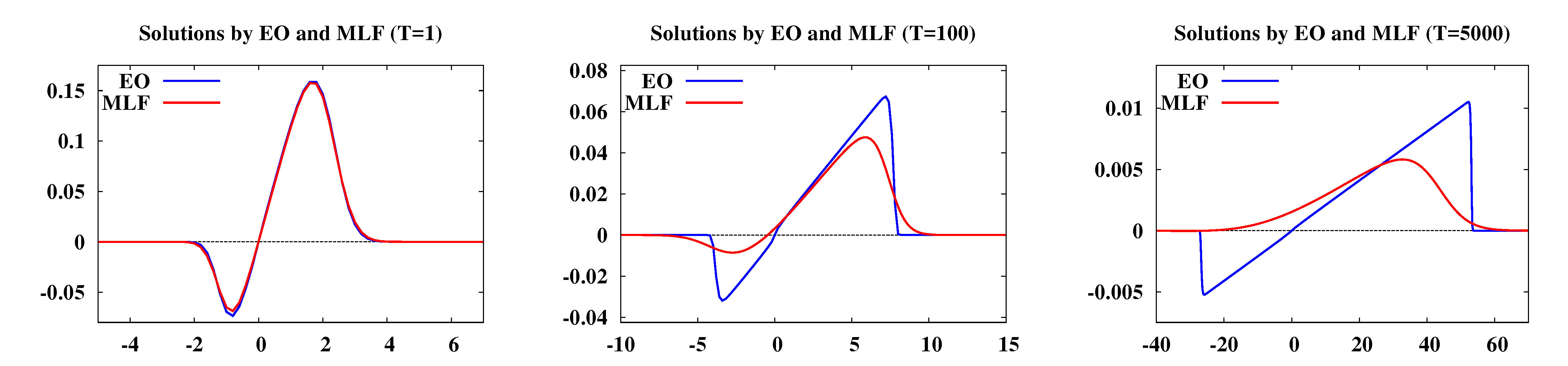Figure 1: Solutions of (2) with $\nu=10^{-6}$ at $t=1$, $t=100$ and $t=5000$, using (3) with ${\Delta x}=0.2$, ${\Delta t}=0.5$ and numerical fluxes EO (blue) and MLF (red).

The main aim of our work is to emphasize that ignoring the dynamics of the continuous model at the numerical level can produce undesired results in optimal control problems in large time horizons. On one hand, we show that the gradient descent method performs successfully whenever the numerical flux and the mesh sizes are chosen appropriately. On the other hand, we present examples where excessive numerical viscosity dominates the physical one.

---