Download Code
In [1], we discuss several aspects of wave propagation in a computational
framework. In particular, we consider the following one-dimensional wave equation
and we discuss the propagation properties of its finite-difference solutions on uniform and non-uniform grids, by establishing comparisons with the usual behavior of the continuos waves.
Our approach is based on the study of the propagation of high-frequency Gaussian beam solutions (that is, solutions originated from highly concentrated and oscillating initial data), both in continuous and
discrete media.
Roughly speaking, the idea at the basis of this techniques is that the energy of Gaussian beam solutions propagates along bi-characteristic rays, which are obtained from the Hamiltonian system associated to the
symbol of the operator under consideration.
At the continuous level of equation \eqref{main_eq_1d}, these mentioned rays are straight lines and travel with a uniform velocity.
On the other hand, the finite difference space semi-discretization of \eqref{main_eq_1d} may introduce different dynamics, with a series of unexpected propagation properties at high frequencies. For instance, one can generate spurious solutions traveling at arbitrarily small velocities which, therefore, show lack of propagation in space.
In addition, the introduction of a non-uniform mesh for the discretization may generate further pathologies such as internal
reflections, meaning that the waves change direction without hitting the boundary.
In order to illustrate these mentioned pathological phenomena, we perform simulations on a uniform space-mesh of $N$ points and mesh-size $h=2/(N+1)$
and on two non-uniform ones produced by applying to $\mathcal G_h$ the transformations
Moreover, the initial data are constructed starting from the following Gaussian profile
Low frequency simulations
We present in Figure 1 our simulations for low-frequency solutions of \eqref{main_eq_1d}. In particular, we considered initial position and frequency $(x_0,\xi_0)=(0,\pi/4)$ and a time horizon $T=5s$.
In this case, the numerical solutions behave basically like the continuous ones: they start traveling to the left along the straight characteristic line $x+t$ and, after having hit the boundary, they reflect following the Descartes-Snell’s law and continue propagating, this time to the right along the other branch of the characteristic ($x−t$).
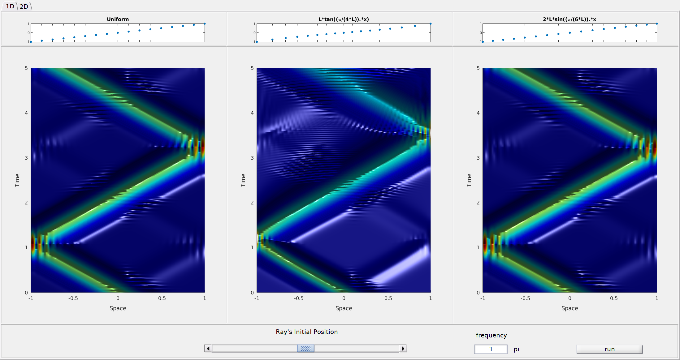
Figure 1. Numerical solutions of \eqref{main_eq_1d} with $(x_0,\xi_0)=(0,\pi/4)$ on uniform and non-uniform meshes.
High frequency simulations
When increasing the frequency, the situation changes and we encounter several interesting phenomena and pathologies:
• The so-called umklapp or U-process, also known as internal reflection, consisting in the reflection of waves without touching only one or both the endpoints of the space interval. This phenomenon is typical for the semi-discretization of high-frequecncy solutions of \eqref{main_eq_1d} on non-uniform meshes, which may produce waves oscillating in the interior of the computational domain and reflecting without touching the boundary (see Figure 2 - middle) or touching the boundary only at one of the endpoints (see Figure 2 - right).
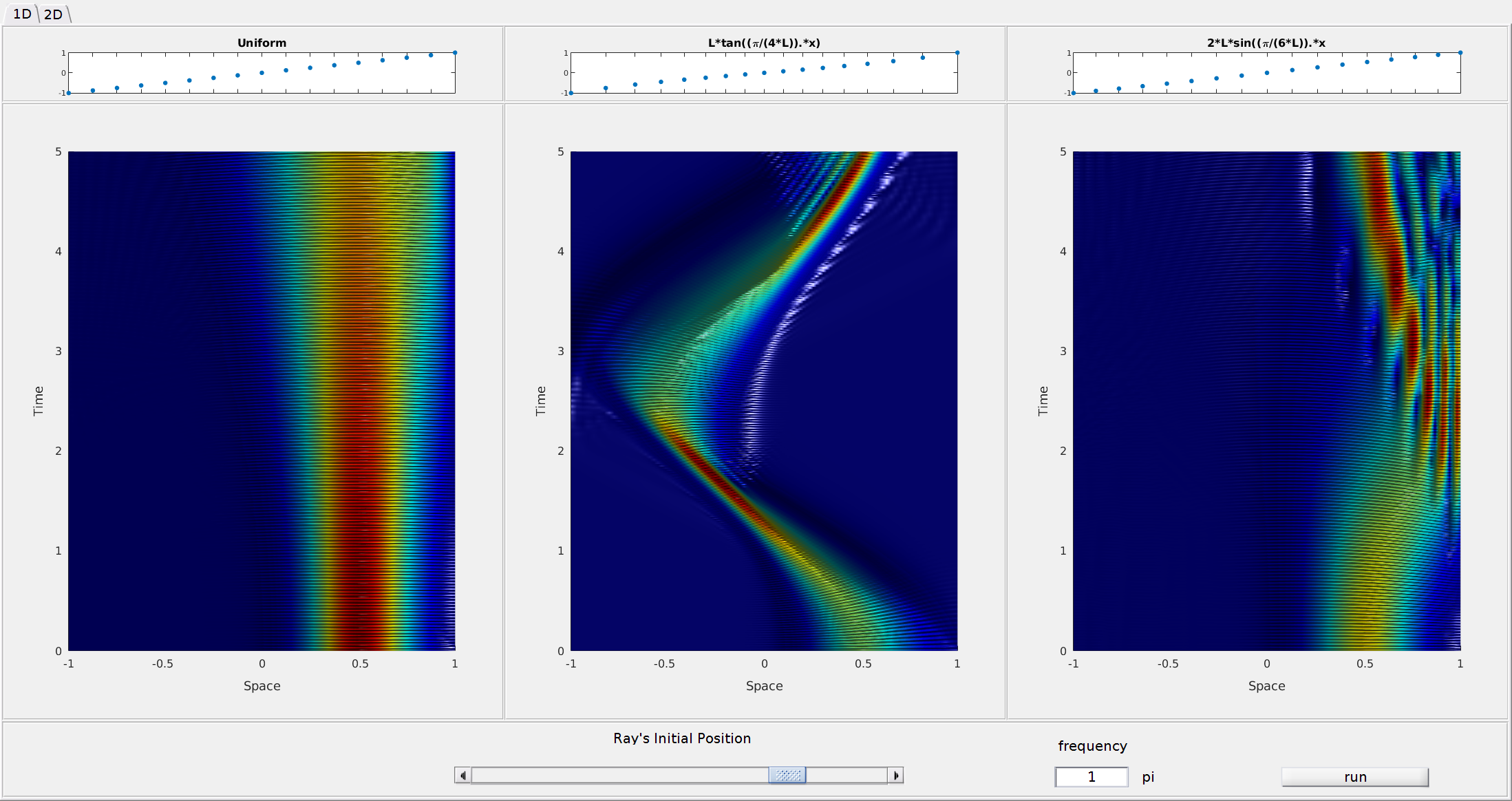
Figure 2. Numerical solutions of \eqref{main_eq_1d} with $(x_0,\xi_0)=(1/2,\pi)$ on uniform and non-uniform meshes.
• Non-propagating waves, corresponding to equilibrium (fixed) points on the phase diagram (see Figure 3).
Figure 3. Numerical solutions of \eqref{main_eq_1d} with $(x_0,\xi_0)=(0,\pi)$ on uniform and non-uniform meshes.
These phenomena are related with the particular nature of the discrete group velocity which, in the finite difference setting, is given by
and vanishes for $\xi = (2k+1)\pi$, $k\in\mathbb{Z}$. Moreover, they can be understood by looking at the phase portrait of the hamiltonian system associated to the finite difference semi-discretization of \eqref{main_eq_1d} (see Figure 4).
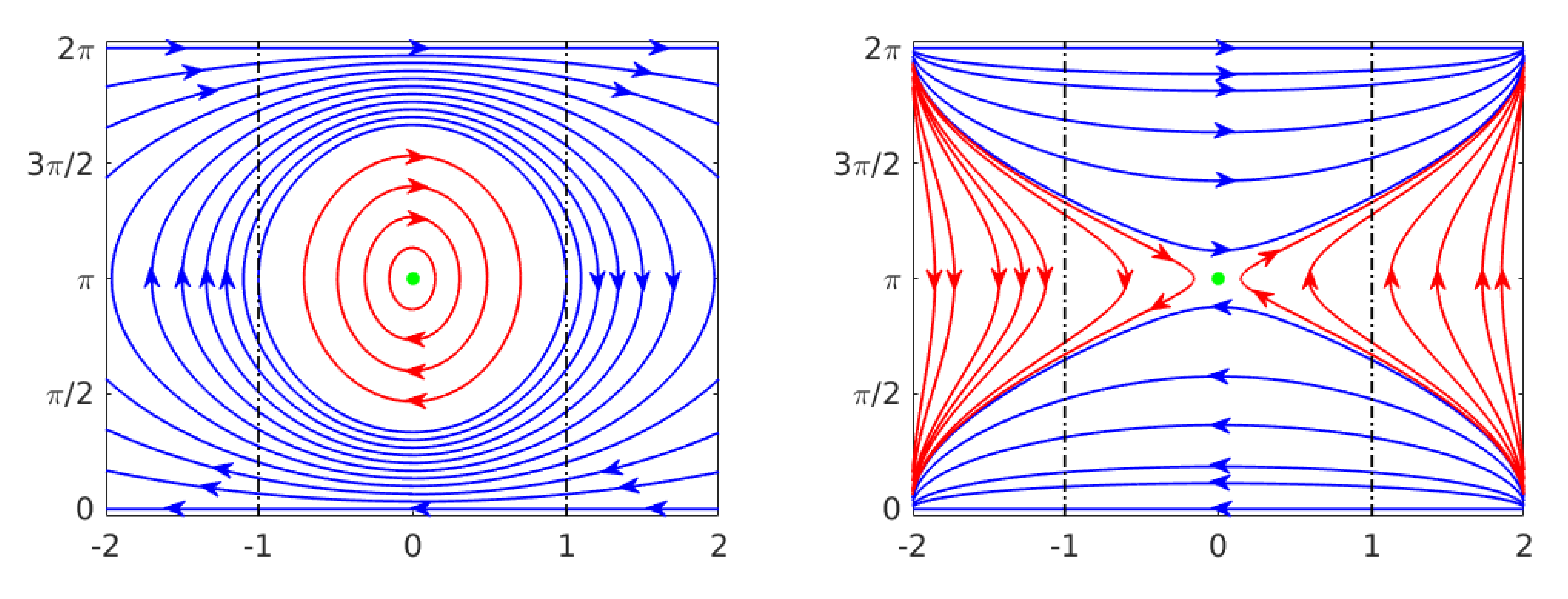
Figure 4. Phase portrait of the Hamiltonian system for the numerical wave equation corresponding to the and the grid transformation $g_1$ (left) and $g_2$ (right).
In particular, the solutions displayed in Figure 2 correspond to
trajectories which remain always in the red area of these phase portraits, while Figure 3 shows solutions starting from the equilibrium point $(0,\pi)$ (the green one in Figure 4)
Notice that, for the grid transformation $g_1$, this equilibrium point is a center (stable) while it is a saddle (unstable) for the grid transformation $g_2$. For this reason, in the first case the non-propagating wave remains concentrated along the vertical ray, while in the second case the wave presents more very dispersive features.
Two-dimensional simulations
Analogous phenomena can be detected also in the case of the finite-difference semi-discretization of the two-dimensional wave equation
Also in this case, we perform simulations on a uniform mesh of $N$ points both in the $x$ and $y$ direction and mesh-sizes $h_x=2/(N+1)=h_y$
and on two non-uniform ones produced by applying to $\mathcal G_h$ the transformations $g_1$ and $g_2$ above introduced.
Moreover, the initial data are constructed once again starting from a Gaussian profile:
Then, it can be observed in Video 1 that, as for the one-dimensional case, at low frequencies the solution remains concentrated and propagates along straight characteristics which reach the boundary, where there is reflection according to the Descartes-Snell’s law. This independently on whether we use a uniform or a non-uniform mesh.

Video 1. Numerical solutions of \eqref{main_eq_2d} with $(x_0,y_0,\xi_0,\eta_0)=(0,0,\pi/4,\pi/4)$ on uniform and non-uniform meshes.
Nevertheless, increasing the frequencies similar phenomena as in the one-dimensional case show up. For instance, on the non-uniform mesh corresponding to the transformation $g_1$, we observe the so-called
rodeo effect, according to which, waves that should propagate along straight lines are trapped along closed circles (Video 2 - middle).
Video 2. Numerical solutions of \eqref{main_eq_2d} with $(x_0,y_0,\xi_0,\eta_0)=(0,\tan(\arccos(\sqrt[4]{1/2},\pi/2,\pi)$ on uniform and non-uniform meshes.
Finally, waves starting from the point $(x_0,y_0,\xi_0,\eta_0)=(0,0,\pi,\pi)$, which is an equilibrium for the phase Hamiltonian system, cannot move, and remain trapped around the point $(0,0)$ in the physical plane for any time (see Video 3).
Video 3. Numerical solutions of \eqref{main_eq_2d} with $(x_0,y_0,\xi_0,\eta_0)=(0,0,\pi,\pi)$ on uniform and non-uniform meshes.
Conclusions
Summarizing, our analysis shows that the finite-difference semi-discretization of one and two-dimensional waves may modify the dynamics of the continuous model. In particular, as a result of the accumulation of the local effects introduced by the heterogeneity of the employed grid, numerical high-frequency solutions can bend in a singular and unexpected manner. Moreover, this phenomenon has to be added to the well known numerical dispersion effect, producing the high-frequency discrete group velocity to vanish, even in uniform grids.
Our results constitute a warning both for adaptivity and for the treating of control and inverse problems. In broad terms, the goal of adaptivity is to refine a mesh on the support of the solution, keeping it coarse where the solution has little oscillations and energy. Our analysis shows that, in this context, adaptivity has to be performed with some attention. Indeed, if one is not careful enough when refining the mesh, they can be produced spurious effects due to the fact that waves feel the fictitious numerical boundaries that are generated when the grid passes from fine to coarse. Finally, our results are also a signal that the dangers of uniform meshes in the study of numerical control and inverse problems (already observed in [2]) may be enhanced when the mesh is non-uniform. In more details, the heterogeneity of the grid may introduce added trapping effects, which need to be avoided in
order to prove convergence in the context of controllability, stabilization or inversion algorithms.
References
[1] U. Biccari, A. Marica and E. Zuazua, Propagation of one and two-dimensional discrete waves under finite difference approximation. Submitted
[2] E. Zuazua, Propagation, observation, control and numerical approximation of waves. SIAM Rev. 47, 2 (2005), 197-243.