Multilevel Selective Harmonic Modulation via Optimal Control

Selective harmonic Modulation (SHM) [1,2] is a well-known methodology in power electronics engineering, employed to improve the performance of a converter by controlling the phase and amplitude of the harmonics in its output voltage. As a matter of fact, this technique allows to increase the power of the converter and, at the same time, to reduce its losses.

In broad terms, SHM consists in generating a control signal with a desired harmonic spectrum by modulating some specific lower-order Fourier coefficients. In practice, the signal is constructed as a step function with a finite number of switches, taking values only in a given finite set. Such a signal can be fully characterized by two features (see Fig. 1):

1. The waveform, i.e. the sequence of values that the function takes in its domain.
2. The switching angles, i.e. the sequence of points where the signal switches from one value to following one.

In mathematical terms, the SHM problem can be formulated as follows. Let

$$\begin{equation}\label{eq:Udef} \mathcal{U} = \{u_1, \ldots, u_L\} \end{equation}$$

be a given set of $L\geq 2$ real numbers satisfying $u_1 = -1$, $u_L = 1$ and $u_k<u_{k+1}$ for all $k\in {1,\ldots, L}$.

The goal is to construct a step function $u(t):[0,2\pi)\to\mathcal U$ with a finite number of switches, such that some of its lower-order Fourier coefficients take specific values prescribed a priori.

Due to applications in power converters, it is typical to only consider functions with half-wave symmetry, i.e. satisfying $u(t + \pi) = -u(t)$ for all $t \in [0,\pi)$.

In view of this symmetry, the Fourier series of $u$ only involves the odd terms (as the even terms just vanish), i.e.

$$u(t) = \sum_{\underset{j\, odd}{j \in \mathbb{N}}} a_j \cos(jt)+ \sum_{\underset{k\, odd}{j \in \mathbb{N}}} b_j \sin(jt),$$

with

$$a_j = \frac{2}{\pi} \int_0^\pi u(\tau ) \cos(j \tau)\,d\tau \quad$$

and

$$b_j = \frac{2}{\pi} \int_0^\pi u(\tau) \sin(j \tau)\,d\tau.$$

Moreover, the functions we are considering are piecewise constant with a finite number of switches, taking values only in $\mathcal{U}$, i.e. of the form

$$\begin{equation}\label{eq:uExpl} u (t)= \sum_{m=0}^M s_m\chi_{[\phi_m,\phi_{m+1})} (t), \quad M\in\mathbb{N} \end{equation}$$

for some $\mathcal S = {s_m}_{m=0}^M$ satisfying

$$s_m\in \mathcal{U} \; \text{ and } \; s_m\neq s_{m+1}, \quad \forall\, m\in \{0,\ldots, M\}$$

and $\Phi = {\phi_m}_{m=1}^{M}$ such that

$$0= \phi_0 < \phi_1 <\ldots < \phi_M < \phi_{M+1} = \pi .$$

Here $\mathcal S$ and $\Phi$ are the waveform and the switching angles that we mentioned above.

Observe that any function $u$ of the form \eqref{eq:uExpl} is fully characterized by its waveform $\mathcal S$ and switching angles $\Phi$. An example of such a function is displayed in Fig. 1

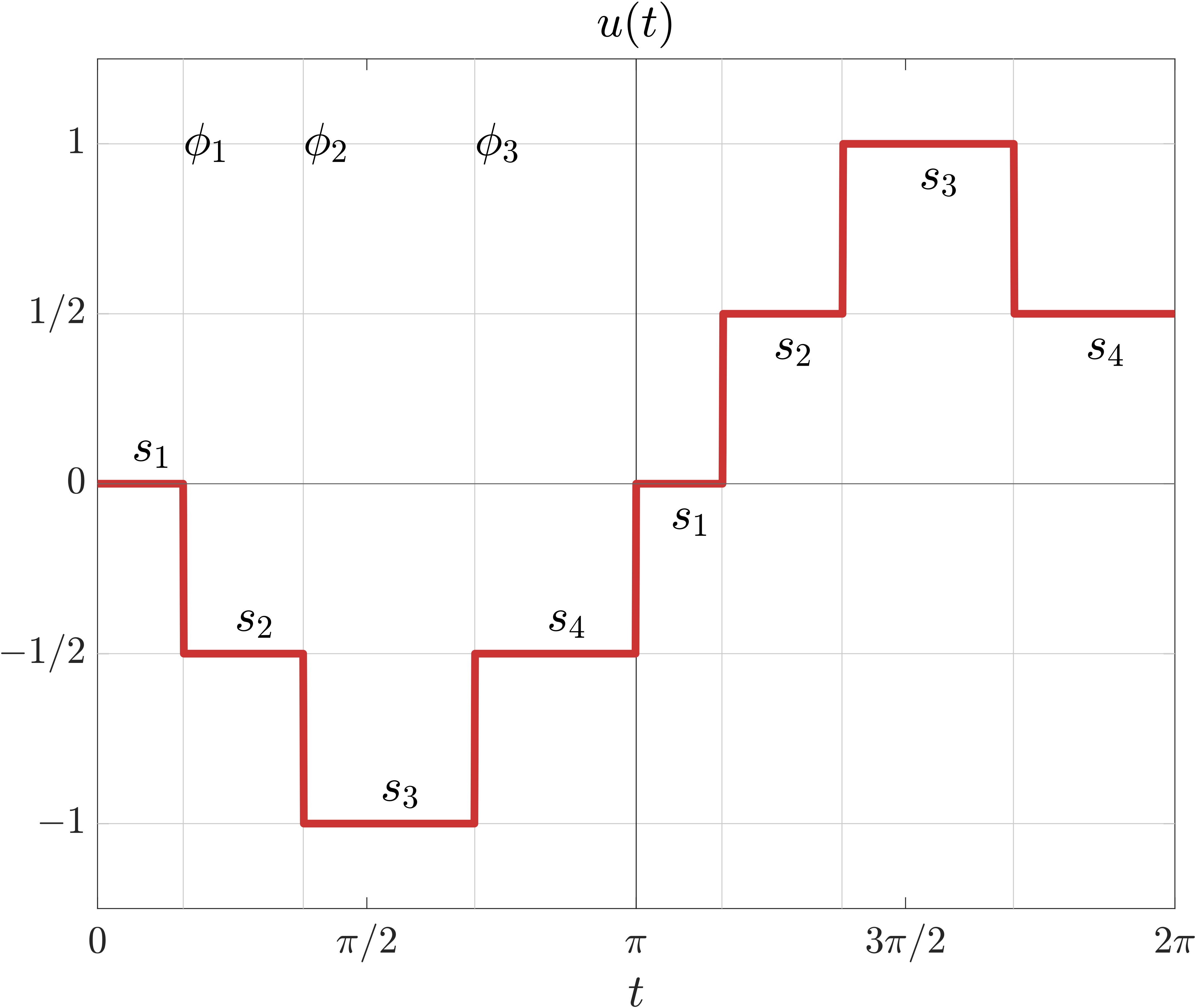Figure 1: a possible solution to the SHM Problem, where we considered the control-set $\mathcal{U} = \{-1, -1/2, 0, 1/2, 1\}$. We show the switching angles $\Phi$ and the waveform $\mathcal S$. The function $u(t)$ is displayed on the whole interval $[0,2\pi)$ to highlight the half-wave symmetry.

In practical engineering applications, due to technical limitations, it is preferable to employ signals taking consecutive values in $\mathcal{U}$. This property of the waveform, to which we shall refer as the staircase property, can be rigorously formulated as follows:

Definition: We say that a signal $u$ of the form \eqref{eq:uExpl} fulfills the staircase property if its waveform $\mathcal S$ satisfies

$$\begin{equation}\label{eq:staircase prop} \begin{array}{l} (s_m^{min},s_{m}^{max}) \cap \mathcal{U} = \emptyset, \quad\forall\, m\in \{ 0, \ldots, M-1 \}, \\[10pt] s^{min}_m = s_m\wedge s_{m+1} \\[10pt] s^{max}_m = s_m \vee s_{m+1} \end{array} \end{equation}$$

We can now formulate the SHM problem as follows.

SHM problem: let $\mathcal{U}$ be given as in \eqref{eq:Udef}, and let $\mathcal E_a$ and $\mathcal E_b$ be finite sets of odd numbers of cardinality $\vert\mathcal{E}_a\vert=N_a$ and $\vert\mathcal{E}_b\vert=N_b$ respectively. For any two given vectors $a^T\in\mathbb{R}^{N_a}$ and $b^T\in\mathbb{R}^{N_b}$, construct a function $u:[0,\pi)\to\mathcal{U}$ of the form \eqref{eq:uExpl}, satisfying \eqref{eq:staircase prop}, such that the vectors

$$a=(a_j)_{j\in\mathcal{E}_a} \quad\quad b=(b_j)_{j\in\mathcal{E}_b}$$

satisfy $a = a^T$ and $b = b^T$.

SHM as an optimal control problem

To solve the SHM problem, in [3] we propose an optimal control-based approach in which the Fourier coefficients of the signal $u(t)$ are identified with the terminal state of a controlled dynamical system of $N_a+N_b$ components defined in the time-interval $[0,\pi)$. The control of the system is precisely the signal $u(t)$, defined as a function $[0,\pi)\to \mathcal{U}$, which has to steer the state from the origin to the desired values of the prescribed Fourier coefficients.

The starting point of this approach is to rewrite the Fourier coefficients of the function $u(t)$ as the final state of a dynamical system controlled by $u(t)$. To this end, let us first note that, by definition, for all $u\in L^\infty ([0,\pi);\mathbb{R})$ any Fourier coefficient $a_j$ satisfies $a_j = y(\pi)$, with $y\in C([0,\pi);\mathbb{R})$ defined as

$$y(t) = \dfrac{2}{\pi} \int_0^t u(\tau) \cos(j\, \tau) d\tau.$$

Besides, as a consequence of the fundamental theorem of calculus, $y(\cdot)$ is the unique solution to the differential equation

$$\begin{cases} \dot{y} (t) = \dfrac{2}{\pi} \cos(j\, t) u(t), \qquad t\in [0,\pi) \\[5pt] y(0) = 0. \end{cases}$$

Analogously, we can also write the Fourier coefficients $b_j$ as the solution at time $t=\pi$ of a similar differential equation.

Hence, for $\mathcal{E}_a$, $\mathcal{E}_b$, $a^T$, and $b^T$ given, the SHM Problem can be reduced to finding a control function $u$ of the form \eqref{eq:uExpl}, satisfying \eqref{eq:staircase prop}, such that the corresponding solution $\textbf{y}\in C([0,\pi);\mathbb{R}^{N_a+N_b})$ to the dynamical system

$$\begin{cases} \dot{\textbf{y}}(t) = \dfrac{2}{\pi} \mathcal{D}(t) u(t), \qquad t\in [0,\pi) \\[5pt] \textbf{y}(0) = 0 \end{cases}$$

satisfies $\textbf{y}(\pi) = [a^T;b^T]^\top$, where

$$\mathcal{D}(t) = \left[\mathcal{D}^a(t);\mathcal{D}^b(t) \right]^\top,$$

with $\mathcal{D}^a(t) \in \mathbb{R}^{N_a}$ and $\mathcal{D}^b(t) \in \mathbb{R}^{N_b}$ given by

$$\mathcal{D}^a(t) = \begin{bmatrix} \cos(e_a^1t) \\ \cos(e_a^2t) \\ \vdots \\ \cos(e_a^{N_a}t) \end{bmatrix}, \quad \mathcal{D}^b(t) = \begin{bmatrix} \sin(e_b^1t) \\ \sin(e_b^2t) \\ \vdots \\ \sin(e_b^{N_b}t) \end{bmatrix}$$

Here, $e_a^i$ and $e_b^i$ denote the elements in $\mathcal{E}_a$ and $\mathcal{E}_b$, i.e. $\mathcal{E}_a = \{e_a^1,e_a^2,e_a^3,\dots,e_a^{N_a}\}, \quad \mathcal{E}_b = \{e_b^1,e_b^2,e_b^3,\dots,e_b^{N_b}\}.$

Moreover, we can reverse the time using the transformation $\textbf{x} (t) = \textbf{y}(\pi - t)$, so that the SHM problem turns into the following null controllability one, for a dynamical system with initial condition $\textbf{x}(0) = [a^T;b^T]^\top$.

SHM problem via null controllability: let $\mathcal{U}$ be given as in \eqref{eq:Udef}. Let $\mathcal{E}_a$, $\mathcal{E}_b$ and the targets $a^T$ and $b^T$ be given. We look for a function $u: [0,\pi)\to [-1,1]$ of the form \eqref{eq:uExpl}, satisfying \eqref{eq:staircase prop}, such that the solution to the initial-value problem

$$\begin{equation}\label{eq:CauchyReversed} \begin{cases} \displaystyle\dot{\textbf{x}}(t) = -\frac 2\pi\mathcal{D}(t)u(t), & t \in [0,\pi) \\[5pt] \textbf{x}(0) = \textbf{x}_0 := [a^T; b^T] \end{cases} \end{equation}$$

satisfies $\textbf{x} (\pi) = 0$.

A natural approach for null controllability problems is to formulate them as optimal control ones. In the case of the SHM problem just presented, in [3] we proposed to obtain the optimal control $u$ in the following way.

Penalized OCP for SHM: fix $\varepsilon>0$ and a convex function $\mathcal{L}\in C([-1,1];\mathbb{R})$. Let $\mathcal{E}_a$, $\mathcal{E}_b$ and the targets $a^T$ and $b^T$ be given, and denote

$$\mathcal A:=\big\{ u:[0,\pi)\to [-1,1]\;\text{measurable}\,\big\}.$$

We look for a control $u\in \mathcal A$ solution to the following optimal control problem:

$$\begin{array}{l} \displaystyle\min_{u \in \mathcal A}\;\left(\dfrac{1}{2} \|\textbf{x}(\pi)\|^2 + \varepsilon \displaystyle\int_0^\pi \mathcal{L}(u(t)) dt\right) \\[20pt] \text{subject to the dynamics \eqref{eq:CauchyReversed}}. \end{array}$$

Observe that in the above formulation we do not impose the constraint that the control has to be of the form \eqref{eq:uExpl}, satisfying the staircase property \eqref{eq:staircase prop}. These features of $u$ will arise naturally from a suitable choice of the penalization term $\mathcal{L}$, as we describe below.

Bi-level SHM problem via OCP (Bang-Bang Control)

In this case, the control set $\mathcal{U}$ defined in \eqref{eq:Udef} has only two elements, i.e. $\mathcal{U}={-1,1}$. In the control theory literature, a control taking only two values is known as bang-bang control. In the SHM literature, this kind of solution are called bi-level solutions. Moreover, in [3], we proved that bi-level controls are obtained through our optimal control approach when selecting $\mathcal L(u)=\alpha u$ with $\alpha\neq 0$.

Theorem 1: let $L=2$, $\mathcal{U}$ as in \eqref{eq:Udef}, and $\textbf{x}_0$ be given. For some $\alpha\in \mathbb{R}$ with $\alpha\neq 0$, consider the penalization $\mathcal{L} (u) = \alpha\, u$. Then, the optimal control $u^\ast$ is unique and has a bang-bang structure, i.e. it is of the form \eqref{eq:uExpl}. In addition to that, the solution $u^\ast$ is continuous with respect to $\textbf{x}_0$ in the strong topology of $L^1(0,\pi)$.

We point out that the continuity of the solution with respect to the target frequencies is a highly desirable property in real applications of SHM, and sometimes, difficult to achieve.

Multilevel SHM problem via OCP

Another typical situation, known in the power electronics literature as the multilevel SHM problem, is the case when $\mathcal{U}$ contains more than two elements.

In [3], we proved that multilevel controls are obtained when selecting $\mathcal L(u)$ as the interpolate a parabola in $[-1,1]$ by affine functions, considering the elements in $\mathcal{U}$ as the interpolating points.

Theorem 2: let $\textbf{x}_0$ be given, and let $\mathcal{U}$ be a given set as in \eqref{eq:Udef}. For any $\alpha>0$ and $\beta\in \mathbb{R}$, set the function

$$\mathcal{P}(u) = \alpha (u-\beta)^2.$$

Consider the penalization

$$\mathcal{L}(u) = \begin{cases} \lambda_k(u) & \text{if } u \in [u_k,u_{k+1}) \\ \mathcal{P}(1) & \text{if } u = u_{L} \end{cases} \quad \forall\, k \in \{1,\dots,L-1\},$$

where

$$\lambda_k(u):= \dfrac{ (u-u_k)\mathcal{P}(u_{k+1}) + (u_{k+1}- u) \mathcal{P}(u_k)}{u_{k+1} - u_k}.$$

Assume in addition that the function $\mathcal{L}$ has a unique minimum in $[-1,1]$. Then, the optimal control $u^\ast$ is unique and has the form \eqref{eq:uExpl} satisfying \eqref{eq:staircase prop}. Moreover, the solution $u^\ast$ is continuous with respect to $\textbf{x}_0$ in the strong topology of $L^1(0,\pi)$.

The assumption of $\mathcal L$ having a unique minimum in $[-1,1]$ is actually necessary to ensure the staircase form for the solution. Not assuming this hypothesis would entail the possibility of having continuous solutions for specific targets. Nevertheless, this assumption can be easily ensured by choosing, for instance, $\beta = \pm1$.

We illustrate in Fig. 2 different examples of penalization functions $\mathcal{L}$ giving rise to multilevel solutions to the SHM problem. We point out that, by varying the values of $\alpha$ and $\beta$ in $\mathcal P$, we can obtain solutions with different waveforms.

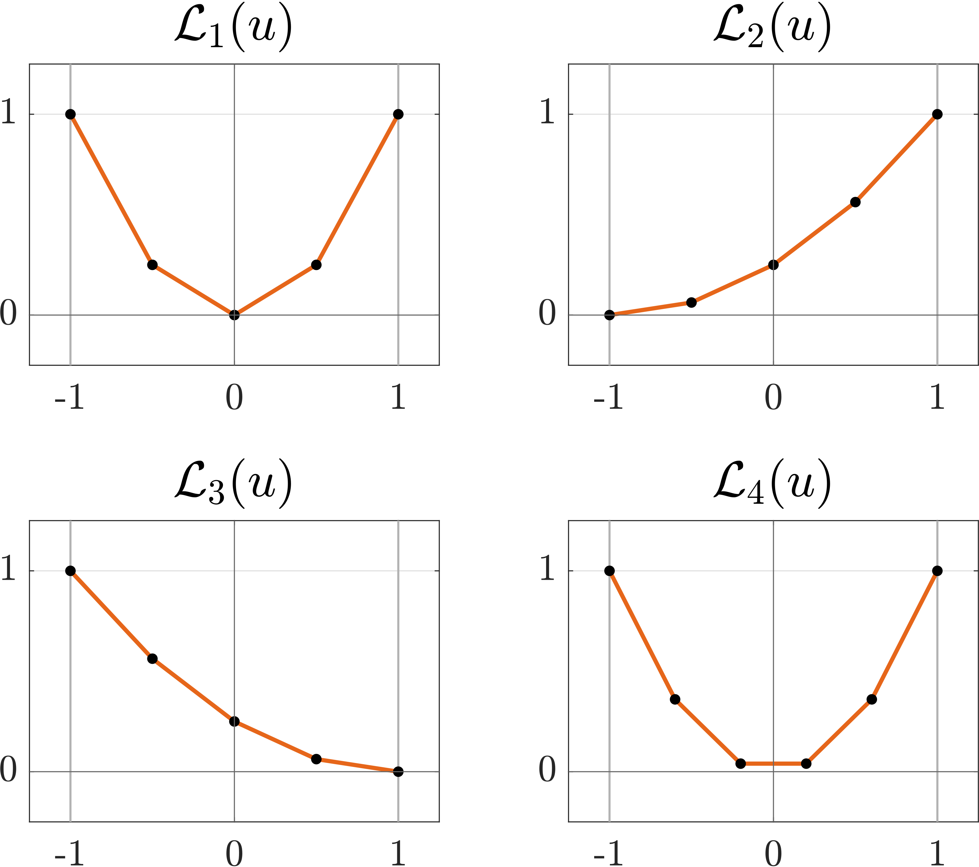Figure 2: some examples of convex piecewise affine penalization functions $\mathcal{L}$. The examples $\mathcal {L}_1$, $\mathcal{L}_2$ and $\mathcal{L}_3$ satisfy the hypotheses of Theorem 2. On the contrary, the function $\mathcal{L}_4$ has not a unique minimizer, and then, we cannot ensure that the solution has staircase form.

Numerical simulations

Let us now present several examples in which we implement the optimal control strategy we proposed to solve the SHM problem.

To solve our optimal control problem, we employ the direct method which, in broad terms, consists in discretizing the cost functional and the dynamics, and then apply some optimization algorithm. The dynamics is approximated with the Euler method, while for solving the discrete minimization problem we employ the nonlinear constrained optimization tool CasADi. CasADi is an open-source tool for nonlinear optimization and algorithmic differentiation which implements the interior point method via the optimization software IPOPT. To be efficiently applied to solve an optimal control problem, we then need the functional we aim to minimize to be smooth. While this is clearly true in the bi-level case, for the multilevel one the functional, due to the piecewise affine penalization, is not differentiable at the points $u_k\in\mathcal U$. For this reason, when treating the multilevel case, we will first need to build a smooth approximation of the function $\mathcal L$.

Smooth approximation of $\mathcal L$ for multilevel control

The piecewise affine function defining the penalization $\mathcal L$ in case of multilevel controls can be regularized as follows.

First of all, for all real parameter $\theta>0$, we define the $C^\infty(\mathbb{R})$ function

$$\displaystyle h^\theta(x) := \frac{1 + \tanh(\theta x)}{2}.$$

and observe that, for almost every $x\in \mathbb{R}$, we have that $h^\theta(x)\to h(x)$ as $\theta\to +\infty$, where $h$ is the Heaviside function

$$h(x) = \begin{cases} 1 & \text{ if } x > 0 \\ 0 & \text{ if } x \leq 0. \end{cases}$$

Secondly, for all $k \in {1,\dots,N_u-1}$ we define the (smooth) function $\chi_{[u_k,u_{k+1})}^\theta:\mathbb{R} \rightarrow \mathbb{R}$ given by

$$\chi_{[u_k,u_{k+1})}^\theta(x) := - 1 + h^\theta(x-u_k) + h^\theta(-x+u_{k+1})$$

which, as $\theta\to +\infty$, converges in $L^\infty(\mathbb{R})$ to the characteristic function $\chi_{[u_k,u_{k+1})}$. Finally, we employ $\chi_{[u_k,u_{k+1})}^\theta$ to define

$$\mathcal{L}^\theta(u) = \sum_{k = 1}^{N_u-1} \lambda_k \chi^\theta_{[u_k,u_{k+1})}(u)$$

which, as $\theta\to +\infty$, converges in $L^\infty(\mathbb{R})$ to the penalization function $\mathcal L$ we defined for multilevel control.

Direct method for OCP-SHE

The starting point for employing a direct method to solve the optimal control problem we are considering is to discretize the cost functional and the dynamics. To this end, let us consider a $N_t$-points partition of the interval $[0,\pi]$, $\mathcal{T} = {t_k}_{k=1}^{N_t}$, and denote by $\textbf{u} \in \mathbb{R}^{N_t}$ the vector with components $u_k = u(t_k)$, $k=1,\ldots,N_t$.

Then the optimal control problem can then be approximated by a finite-dimensional optimization one with variable $\textbf{u} \in \mathbb{R}^{N_t}$.

Numerical OCP: given two sets of odd numbers $\mathcal{E}_a$ and $\mathcal{E}_b$ with cardinalities $\vert\mathcal{E}_a\vert=N_a$ and $\vert\mathcal{E}_b\vert=N_b$, respectively, the target vectors $a^T\in\mathbb{R}^{N_a}$ and $b^T\in\mathbb{R}^{N_b}$, and the partition $\mathcal{T}$ of the interval $[0,\pi]$, we look for $\textbf{u}\in\mathbb{R}^{N_t}$ that solves the following minimization problem:

$$\begin{equation*} \begin{array}{l} \min_{\textbf{u}\in\mathbb{R}^{N_t}} \Bigg[\| \textbf{x}_{N_t}\|^2 + \varepsilon \sum_{k=1}^{N_t-1} \bigg[\frac{\mathcal{L}^\theta(u_{t_k}) + \mathcal{L}^\theta(u_{t_{k+1}})}{2}\Delta t_k \bigg] \Bigg] \\[25pt] \text{subject to: } \begin{cases} \textbf{x}_{t_{k+1}} = \textbf{x}_{t_k} - \Delta t_{k} (2/\pi) \mathcal{D}(t_k)\\[5pt] \textbf{x}_{t_1} = \textbf{x}_0:= [a^T,b^T]^\top \end{cases} \end{array} \end{equation*}$$

where

$$\Delta t_{k} = t_{k+1} - t_{k}, \hspace{1em} \forall\, k \in \{1,\dots,N_t-1\}.$$

Numerical experiments

We now present several numerical experiments to show the effectiveness of our optimal control approach to solve SHM problems. All the examples share the following common parameters $\varepsilon = 10^{-5}, \quad \theta = 10^5, \quad \text{and} \quad\mathcal{P}_t = \{0,0.1,0.2,\dots,\pi\}.$ We consider the frequencies $\mathcal{E}_a = \mathcal{E}_b = \{1,5,7,11,13\},$ and the target vectors $a^T = b^T = (m,0,0,0,0,0)^\top, \quad \forall\, m \in [-0.8,0.8].$

We shall consider three different control sets $\mathcal{U}$ which correspond to different types of control:

• Bang-bang control: $\mathcal{U} = \{-1,1\}$.
• Bang-off-bang control: $\mathcal{U} = \{-1,0,1\}$.
• 5-multilevel control: $\mathcal{U} = \{-1,-1/2,0,1/2,1\}$.

The results of our simulations are displayed in Fig. 3, 4 and 5. We have plotted the function

$$\begin{array}{cccc} \Phi: & [-0.8, 0.8]\times [0,\pi] & \longrightarrow & \mathcal{U} \\ & (m, t ) &\longmapsto & u_m^\ast (t), \end{array}$$

where, for each $m \in [-0.8,0.8]$, $u_m^\ast (\cdot)$ represents the solution to the SHM problem with the target frequencies we are considering.

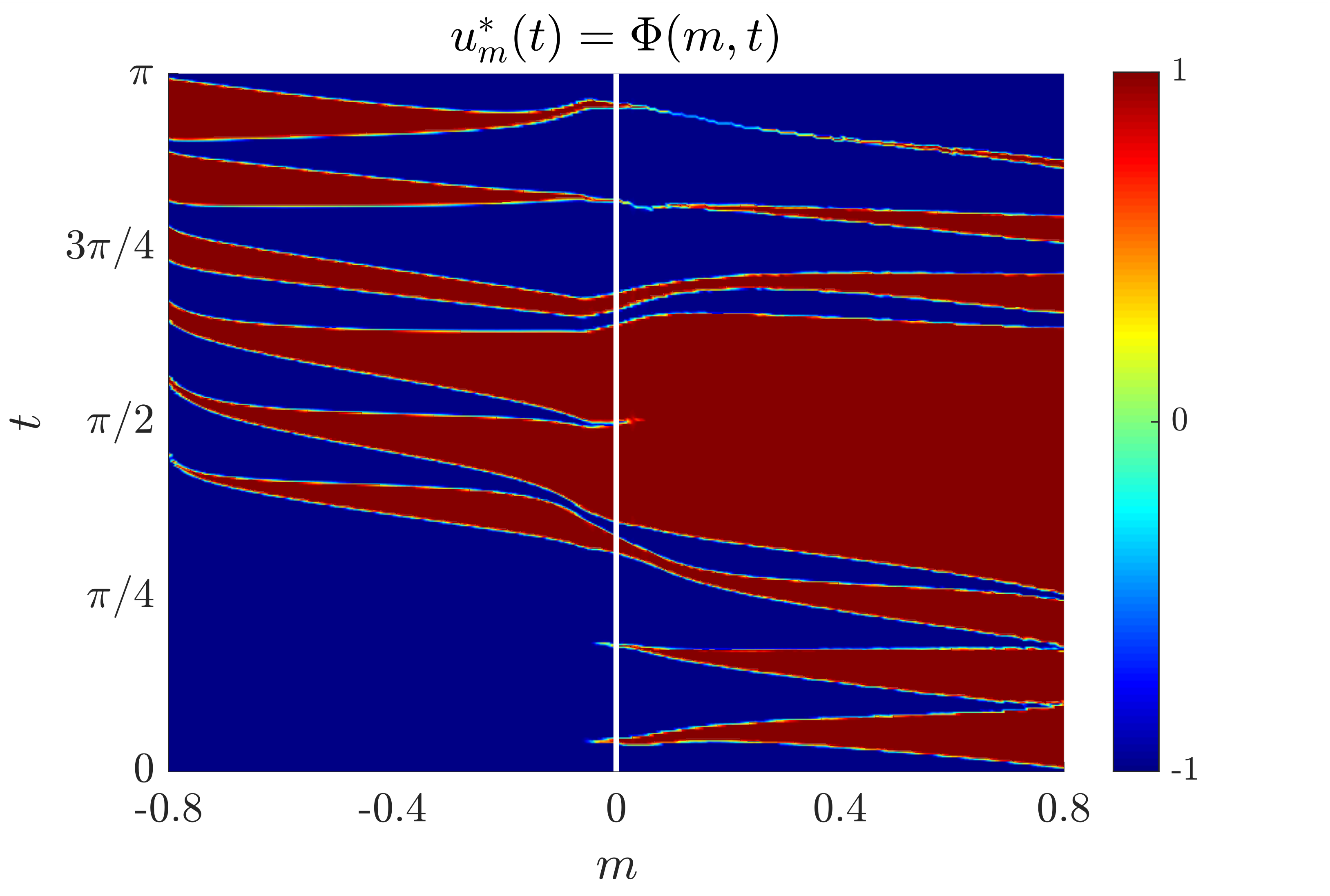Figure 3: bang-bang control for the SHM problem.

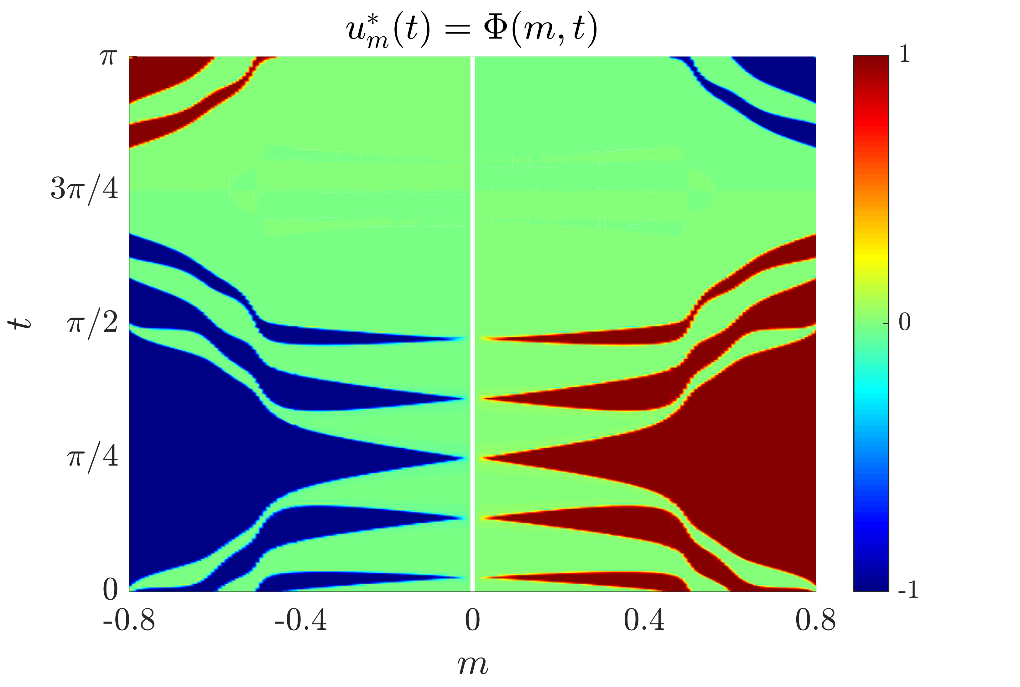Figure 4: bang-off-bang control for the SHM problem.

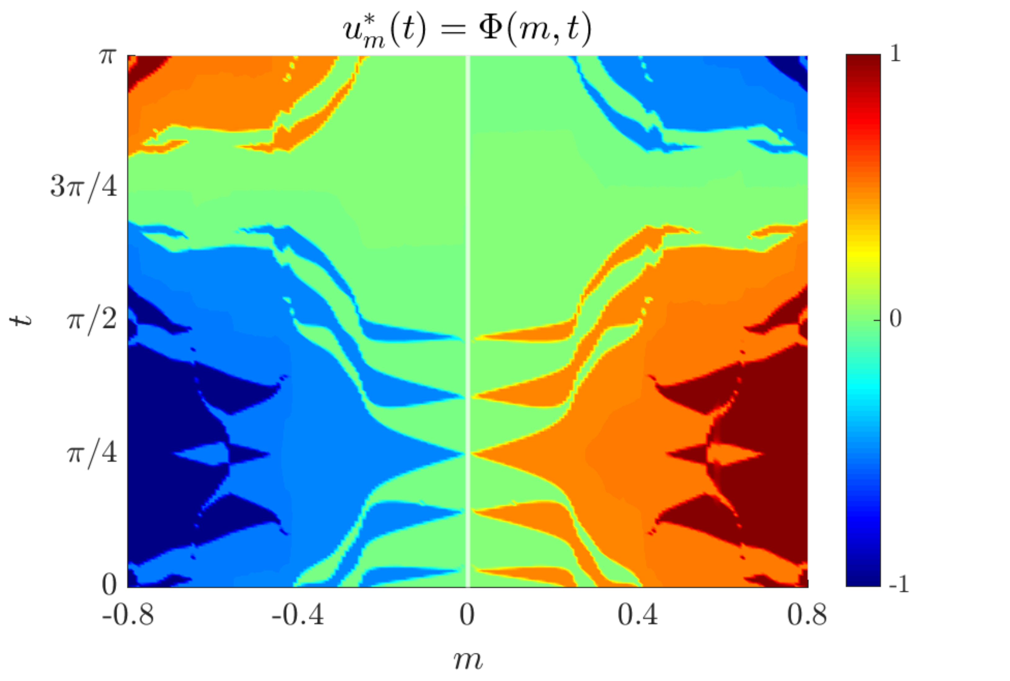Figure 5: multilevel control for the SHM problem.

In Fig. 3, 4 and 5, for each value of the parameter $m$ in the horizontal axis, we observe that the optimal control has the staircase structure. The controls take values only in $\mathcal U$, which are represented by the different colors displayed at the right. For instance, in Fig. 3, the control is $u=-1$ in the blue region and $u=1$ in the red one.

References

[1] J. Sun, S. Beineke and H. Grotstollen Optimal PWM based on real-time solution of harmonic elimination equaations, IEEE Trans. Power Electron., 11(4): 612-621, 1996.

[2] J. Sun and H. Grotstollen Solving nonlinear equations for selective harmonic eliminated PWM using predicted initial values, Proceedings of the 1992 intrenational conference on industrial electronics, control, instrumentation and automation, 1: 259-264.

[3] D. J. Oroya-Villalta, C. Esteve and U. Biccari. Multilevel Selective Harmonic Modulation via Optimal Control, preprint.

---