Download Code
The aim of this tutorial is to give a numerical method for solving an age structured virus model.
Introduction
The virus infection mathematical models are proposing and studying for a long time (see for example C.L. Althaus, R.J. DE Boer [1] and F. Brauer, C. Castillo-Chavez [2]. In particular case of an HIV infection model (see for P. W. Nelson and al. [6]), the corresponding model is usually divided into three classes called uninfected cells, $T$, infected cells, $i$ and free virus particles, $V$.
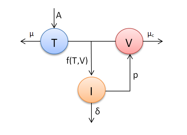
schematic representation of HIV dynamic.
We refer the reader to [4] and [5] for more general class on nonlinear incidence rates that take into account the saturation phenomenon.
We consider an age-structured HIV infection model with a very general nonlinear infection function
with the boundary and initial conditions
We denote by
The number $R_0$ represents the expected number of secondary infections produced by a single infected cell during its lifetime,
The complete global stability analysis for the system (\ref{A}) has been studied in [4]. The system (\ref{A}) admits at most two equilibrium, from Theorem 3.1 and Theorem 5.2 in [4], we obtain the following result:
-
If $R_0 \leqslant 1$, the disease free equilibrium $E_0=(\frac{A}{\mu},0,0)$ is globally asymptotically stable.
-
If $R_0>1$, the positive infection equilibrium $E^{\ast}=(T^\ast,i^\ast,V^\ast)$ is globally asymptotically stable.
Numerical method
We consider the Beddington-Deangelis function $f$ defined by
In this case, the basic reproduction number ${\cal R}_0$ is given by
Where $\pi(a)=\exp^{-\int_{0}^{a} \delta (s) ds}$ and $N=\int_{0}^{\infty} p(a) \pi(a) da$.
The numerical method to solve this system of equation is based on the upwind method for solving hyperbolic partial differential equation, (see [3]) called also the FTBS method (Forward-Time-Backward-Space), has first-order accuracy in both space and time. The CFL condition is necessary for the stability of numerical solutions. The ODEs are solving by explicit Euler method.
we use a grid with points $(x_j,t_n)$ defined by
with age step $\Delta a$ and time step $\Delta t$. Denoting, respectively, by $T^n$, $i^n_j$ and $V^n$ the numerical approximation of $T(t_n)$, $i(t_n,a_j)$ and $V(t_n)$, moreover,
we thus obtain the difference scheme of hyperbolic PDE
with $\lambda = \frac{\Delta t}{\Delta a}$. We fix the following values of parameters
with the initial conditions
The functions $p$ is given by
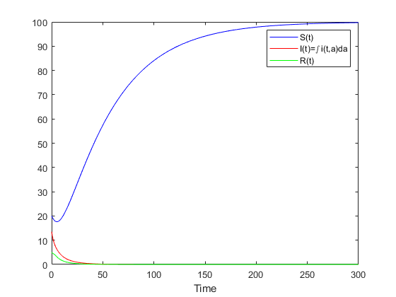
We change the values of $\tau_1$ in order to have $R_0 \leq 1$ or to have $R_0 > 1$. If we choose $ \tau_1 = 3 $ then $ R_0 = 0.5417 < 1 $,
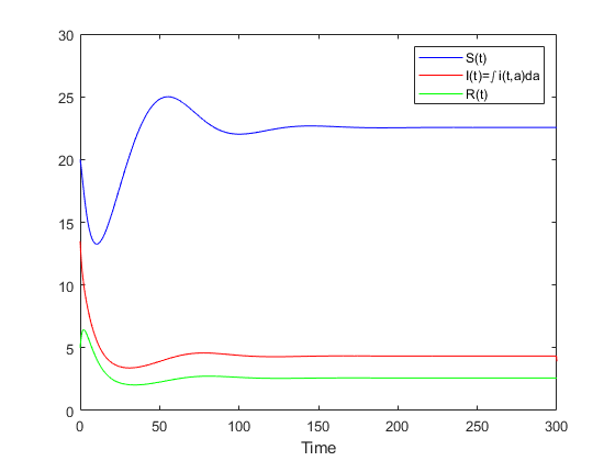
And if we choose $ \tau_1 = 0.5 $ then $ R_0 = 1.4216 > 1 $,
clear all,close all
a1=0;
a2=60;
Tf=300;
I0=@(t)4*exp(-0.3*t);
T0=20;
V0=5;
A0=2; mu=0.02; muc=0.4;
beta=0.1;
alpha1=0.1;
alpha2=0.2;
delta=0.4;
fct=@(x,y) (beta*x*y)/(1+alpha1*x+alpha2*y);
N=199;M=1200;
h=(a2-a1)/N;
k=Tf/M;
a=a1+(1:N)*h;
ap=[0,a];
t=0+(0:M)*k;
lambda=k/h;
C=eye(N);
A=(1-lambda)*C+lambda*diag(ones(1,N-1),-1);
The reproduction number $R_0$
R0=tauxR(N,h,a,delta,beta,muc,mu,A0,alpha1)
T(1)=T0;
V(1)=V0;
U= I0(a(1:N))';  %% initial values
Up=[fct(T0,V0); U]; %% Initial value + Boundary condition
Uf=Up;

F=zeros(N,1);

UI=zeros(1,M);;

for j=1:M
    Uold=U;
      UI(j)=h*fct(T(j),V(j));
    for o=1:N
    UI(j)=UI(j)+h*Uold(o);
    end
    B=[lambda*fct(T(j),V(j)) ;zeros(N-1,1)];
    F=- delta*Uold ;
    U=A*Uold+B+k*F;
    val=feval(@int,Uold,N-1,h,a);
    T(j+1)=T(j)+k*(A0-mu*T(j)-fct(T(j),V(j)));
    V(j+1)=V(j)+k*(val - muc *V(j));
    Up=zeros(N+1,1);
    Up=[fct(T(j+1),V(j+1)); U];
    Uf=[Uf,Up];
end
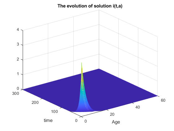
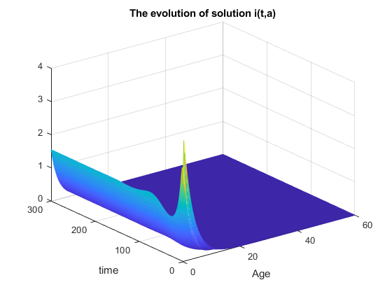
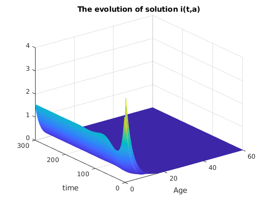
figure(1);
[X , Y] = meshgrid( ap ,t);
mesh (X , Y , Uf')
title('The evolution of solution i(t,a)')
xlabel('Age')
ylabel('time')
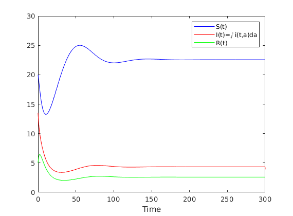
figure(2)
plot(t,T','b',t,[UI UI(N+2)],'r',t,V','g')
legend('S(t)','I(t)=\int i(t,a)da','R(t)')
xlabel('Time')
References
[1] R. J. De Boer C. L. Althaus. Dynamics of immune escape during hiv/siv infection, PloS Comput. Biol, 2008.
[2] F. Brauer and C. Castillo-Chavez. Mathematical Models in Population Biology and Epidemiology Springer, New York, 2000.
[3] L. Edsberg. Introduction to Computation and Modeling for Differential Equations, 2nd Edition. Wiley, 288 Pages, 2016.
[4] M. N. Frioui S. E. Miri, T. M. Touaoula. Unified lyapunov functional for an age-structured virus model with very general nonlinear infection response. J. Appl. Math. Comput, pages 1–27, 2017.
[5] T. Kuniya J. Wang, R. Zhang.. Mathematical analysis for an age-structured hiv infection model with saturation infection rate, Elect. J. Diff. Eq, pages 1–19, 2015.
[6] A. S. Perelson P. W. Nelson. Mathematical analysis of delay differential equation models of hiv-1 infection. Math. Biosc, 179, pages 73–94, 2002.