Download Code
In this tutorial, we will demonstrate how to design a LQR controller in order to stabilize the linear population dynamics model dependent on age and space
where $\beta$ and $\mu$ are respectively the fertility and mortality rate. The parameter $\lambda>0$ is an immigration term (or unstable term), $Q_{\omega}=(a,b)\times (a_1,a_2)\times (0,T)$ is the control domain with $(a,b)\subset (0,1)$ and $(a_1,a_2)\subset (0,A).$ Here $(a,b)=(0,1)$ and $(a_1,a_2)=(0,A)$ and we take $A=1$.
We need to reduce the PDE to the finite dimensional system of the form where $A$ and $B$ are matrices, and
is the finite dimensional state vector.
Implementation
Construction of the matrix A. We suppose that $\lambda=\frac{1}{2}.$
Matrix of birth Here we suppose that fertility rate $\beta$ equal to:
Here $\alpha=7$, $\gamma=5$, $v=3$, $a_1=\frac{A}{9}$
The density of new born individuals will be approximated by:
where $a_i$ is the age discretization.
A1=eye(n);
A2=zeros(n*n,n*n);
for j=m:7*m
    bj=(7*(j/n-1/9)^4*exp(-(j/n-1/9)/3)/(3^5*gamma(5)));
    A2(1:n,(j-1)*n+1:j*n)=bj*A1;
end
P=(25/n)*A2;
Discrerization of the second derivative in space and the derivative in age.
A3=diag(ones(n*n-n,1),-n);
B1=(1/n)*A3;
A4=(-2/(n*n)-1/n)*eye(n);
A5=diag(ones(n-1,1),1);
A6=diag(ones(n-1,1),-1);
B2=A4+(1/(n*n))*A5+(1/(n*n))*A6;
B3=kron(eye(n),B2);
Mortality matrix. The mortality rate $\beta(a)=\dfrac{1}{9(A-a)}$
S=zeros(n*n,n*n);
for j=1:n
    for i=1:n
        S((j-1)*n+i,(j-1)*n+i)=-1/(16*(1-((j*n)/(n*n+1))));
    end
end
A=P+B1+B3+S+(1/2)*eye(n*n);
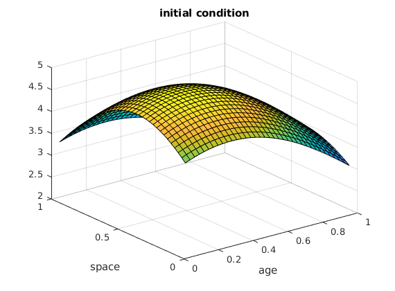
Initial condition
We suppose that $y(x,a,0)=e^{-((a-3/10)^2/\sqrt{2}+100(x-4/10))}$
T=10;
Z0=zeros(n*n,1);
for i=1:n
    for j=1:n
        Z0((i-1)*n+j,1)=5*exp(-((i/n-3/10)^2)/sqrt(2))*exp(-(j/n-4/10)^2);
    end
end
Numerical solution without control and visualisation
f=@(t,Z) A*Z;
[t1,Z]=ode45(f,[0,T],Z0);
L=Z(256,:);
U=Z(512,:);
W=Z(1025,:);
J=reshape(L,n,n);
X=reshape(U,n,n);
Y=reshape(W,n,n);
F1=reshape(Z0,n,n);
V1=linspace(0,1,n+2);
V2=V1(1,2:n+1);
[V3,V4]=meshgrid(V2,V2);
figure;
surf(V3,V4,F1);
xlabel('age');
ylabel('space');
title('initial condition');
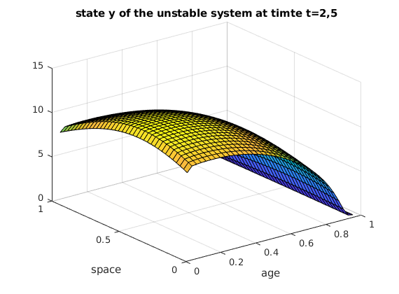
Here is the state y of the unstable system at time t=2,5.
figure;
surf(V3,V4,J);
xlabel('age');
ylabel('space');
title('state y of the unstable system at timte t=2,5');
Here is the state y of the unstable system at time t=5.
figure;
surf(V3,V4,X);
xlabel('age');
ylabel('space');
title('state y of the unstable system at time t=10');
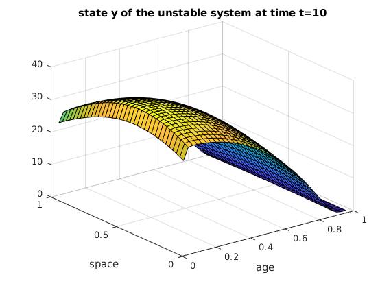
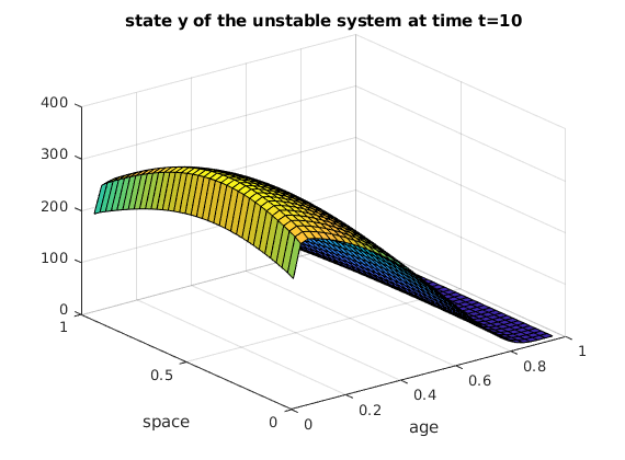
Here is the state y of the unstable system at time t=10.
figure;
surf(V3,V4,Y);
xlabel('age');
ylabel('space');
title('state y of the unstable system at time t=10');
The control matrix B is constructed as follows:
We may now proceed with the optimal control strategy. For a continuous time linear system generated by the matrices $(A,B)$ and an infinite time horizon cost functional defined as
the feedback control law that minimizes the value of the cost is $u = -Kz$, where $K = R^{-1}B*P$ and $P$ is found by solving the continuous time algebraic Ricatti equation
R = eye(n*n); Q = eye(n*n);
H = blkdiag(A, -A');
LQR feedback control-Algebric Ricatti equation
[ricsol, cleig, K, report] = care(A, B, Q, R);
f_ctr = @(z) -K*z;
Numerical solution with LQR feedback control and visualisation
f_2=@(t,Z) A*Z+B*f_ctr(Z);
[t2,Z_ctr]=ode45(f_2,[0,T],Z0);
E=Z_ctr(256,:);
O=Z_ctr(512,:);
G=Z_ctr(1025,:);
G1=reshape(G,n,n);
N=reshape(E,n,n);
M=reshape(O,n,n);
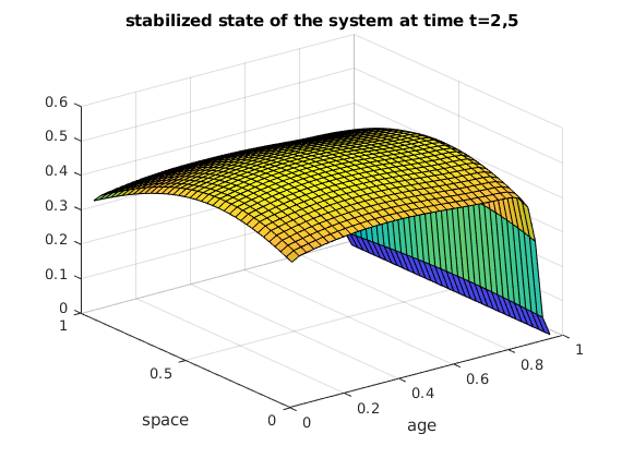
Here is the stabilized state y of the system at the time t=2,5.
figure;
surf(V3,V4,N);
xlabel('age');
ylabel('space');
title('stabilized state of the system at time t=2,5');
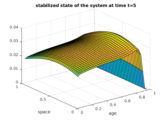
Here is the stabilized state y of the system at time t=5.
figure;
surf(V3,V4,M);
xlabel('age');
ylabel('space');
title('stabilized state of the system at time t=5');
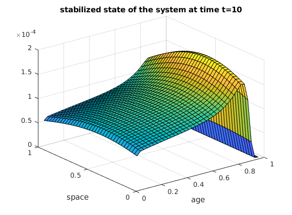
Here is the stabilized state y of the system at time t=10.
figure;
surf(V3,V4,G1);
xlabel('age');
ylabel('space');
title('stabilized state of the system at time t=10')