Download Code
We consider the semilinear hyperbolic system
where $\lambda > 0$ and $u$ is the control. The stability and boundary stabilization of such 1D hyperbolic systems is studied in [1]. The aim of this tutorial is to semi-discretize in space this system of equations and design a stabilizing control by using the LQR method.
The above system linearized around $(y,v) = (0,0)$ has the form
We will first use the LQR method to design a stabilizing control for the semi-discretized linear system, and then this control will be applied to the semi-discretized semilinear system.
Space discretization
The intervall $(0,L)$ is divided in $n+1$ subintervals, of size $h_x := \frac{L}{n+1}$, by $n+2$ evenly spaced points $x_k = kh_x$. Hence, $x_0 = 0$ and $x_{n+1} = L$. We set $y_k(t) = y(x_k,t), \quad v_k(t) := v(x_k,t)$ and similarly for the inital conditions $y_k^0(t) = y^0(x_k)$ and $v_k^0(t) := v(x_k)$.
clear; clc;
L = 1; n = 30;
x = linspace(0, L, n+2);
hx = 1/(n+1);
The points where y and v are unknown are contained in x1 and x2 respectively, where x1 and x2 are defined below.
x1 = x(2:n+2);
x2 = x(1:n+1);
Finite differences for the space derivative give
and
The sign of $\lambda$ in each equation must be taken into account to choose the approximation of $\partial_x y$ and $\partial_x v$.
Let $d = 2(n+1)$ represent the dimension of the state space for the semi-discretized systems. Defining the state variable $z \colon (0,T) \mapsto \mathbb{R}^d$ by
the semilinear system writes as
and the linearized system writes as
We pick the initial condition
y0 = sin(pi*x1)';
v0 = sin(pi*x2)';
z0 = zeros(d, 1); z0(1:n+1, 1) = y0; z0(n+2:d, 1) = v0;
We set values for $\lambda$, $c_1$ and $c_2$:
lambda = 1; c1 = 1; c2 = 1;
We consider the time parameters
T = 5;
nT = 70;
time = linspace(0, T, nT);
The matrix $A$ of size $d \times d$ is given by
where $A_{11}, A_{12}, A_{21}, A_{22}$, of size $(n+1)\times(n+1)$, are defined by
and
They are constructed as follows.
A = zeros(d, d);
%% Lower and upper extradiagonals:
ext_down_1 = zeros(1,2*n+1); ext_down_1(1,1:n) = lambda/hx*ones(1,n);
ext_down_2 = c2*ones(1,n);
ext_up_1 = zeros(1,2*n+1); ext_up_1(1,(n+2):(2*n+1)) = lambda/hx*ones(1,n);
ext_up_2 = zeros(1, n+1); ext_up_2(1, 1) = lambda/hx;
ext_up_3 = c1*ones(1,n);
%% We assemple:
A = A - lambda/hx*eye(d); A(n+2, n+2) = A(n+2, n+2) + c2;
A = A + diag(ext_up_1,1) + diag(ext_up_2, n+1) + diag(ext_up_3,n+2);
A = A + diag(ext_down_1,-1) + diag(ext_down_2, -n-2);
The matrix $B$ is of size $d \times 1$ and is given by
where $B_1, B_2$, of size $(n+1)\times 1$, are defined by
B= zeros(d, 1);
B(n+1, 1) = c1; B(d, 1) = lambda/hx;
The LQR method
We check that a LQR control can be computed for the semi-descretize linear system. To begin, we verify that $ (A,BB^\ast) $ is stabilizable (where $B^\ast$ denotes the transpose of $B$), meaning that $\text{rank}((sI-A) BB^\ast) = d$ for any eigenvalue $s$ of $A$ with a nonnegative real part.
disp('Stabilizability of (A, BB*):');
eA=eig(A);
not_stabilizable = 0;
for cpt=1:d
    if real(eA(cpt))>=0
        disp(cpt); disp(eA(cpt));

        M = zeros(d, 2*d);
        M(:, 1:d) = eA(cpt)*eye(d)-A;
        M(:, d+1:d*2) = B*(B');

        r = rank(M);
        if (r ~= d)
            not_stabilizable = not_stabilizable + 1;
        end
    end
end
if not_stabilizable == 0
    disp('stabilizable.');
else
    disp('not stabilizable.');
end
Stabilizability of (A, BB*):
    18

    0.3047

stabilizable.
Then, we verify that the eigenvalues of the Hamiltonian matrix
are not purely imzginary. Here, $Q$ is a matrix of size $d \times d$ to be chosen.
R = 1; Q = eye(d);
H = blkdiag(A, -A');
H(d+1: 2*d, 1:d) = -Q;
H(1:d, d+1: 2*d) = -B*(B');
eH = eig(H);
nb_imaginary_eig_val_hamiltonian = sum(real(eH) == 0);
disp('Number of eigenvalues of H on the imaginary axis:')
disp(nb_imaginary_eig_val_hamiltonian);
Number of eigenvalues of H on the imaginary axis:
     0
To finish, we verify that $(Q, A)$ is stabilizable, meaning that the rank of
is equal to $d$, for any eigenvalue $s$ of $A$ with a nonnegative real part.
disp('Detectability of (Q, A):');
not_detectable = 0;
for cpt=1:d
    if real(eA(cpt))>=0
        disp(cpt); disp(eA(cpt));

        J = zeros(2*d, d);
        J(1:d, :) = Q;
        J(d+1:d*2, :) = eA(cpt)*eye(d)-A;

        r = rank(J);
        if (r ~= d)
            not_detectable = not_detectable + 1;
        end
    end
end
if not_detectable == 0
    disp('detectable.');
else
    disp('not detectable.');
end
Detectability of (Q, A):
    18

    0.3047

detectable.
The LQR control is given by the matlab routine care(), as the application $t \mapsto -Kz(t)$. The matrix $K$, of size $m \times d$ is an output of care(), where $m$ is the dimention of the input space and is equal to one.
[ricsol, cleig, K, report] = care(A, B, Q, R);
f_ctr = @(z) -K*z;
Unstable and stabilized system’s solutions
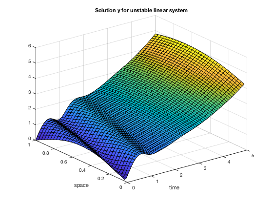
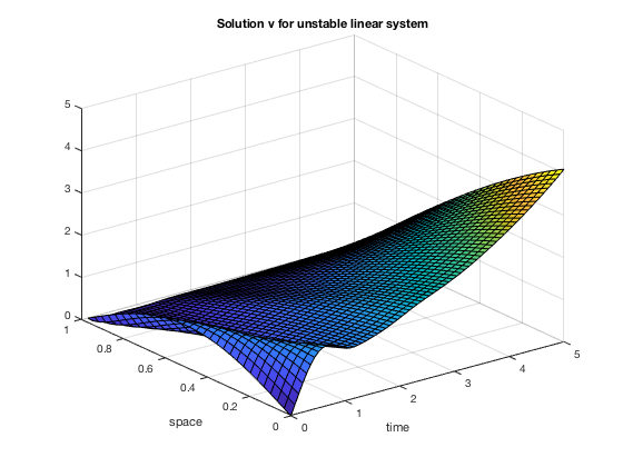
We compute the solution to the linear system with a control equal to zero:
F1 = @(t,z) A*z + B*u;
[t1, Z1] = ode45(F1, time, z0);
The corresponding solutions $y$ and $v$ are displayed:
[X,Y] = meshgrid(t1, x1);
figure; surf(X, Y, Z1(:, 1:n+1)');
xlabel('time'); ylabel('space'); title('Solution y for unstable linear system');

[X,Y] = meshgrid(t1, x2);
figure; surf(X, Y, Z1(:, n+2:2*(n+1))');
xlabel('time'); ylabel('space'); title('Solution v for unstable linear system');
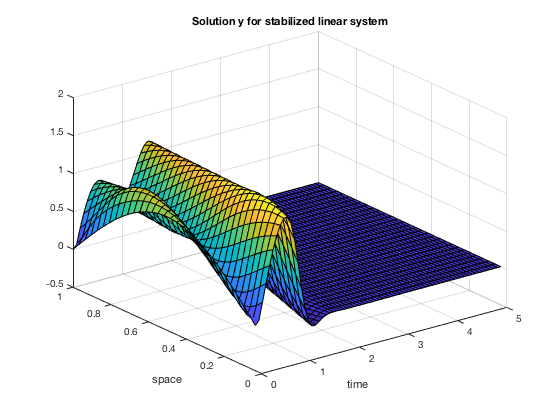
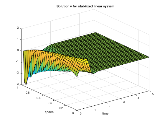
We compute the solution to the linear system with the feedback control:
F2 = @(t,z) A*z + B*f_ctr(z);
[t2, Z2] = ode45(F2, time, z0);
The corresponding solutions $y$ and $v$ are displayed:
[X,Y] = meshgrid(t2, x1);
figure; surf(X, Y, Z2(:, 1:n+1)');
xlabel('time'); ylabel('space'); title('Solution y for stabilized linear system');

[X,Y] = meshgrid(t2, x2);
figure; surf(X, Y, Z2(:, n+2:2*(n+1))');
xlabel('time'); ylabel('space'); title('Solution v for stabilized linear system');
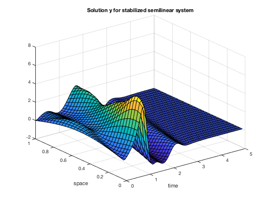
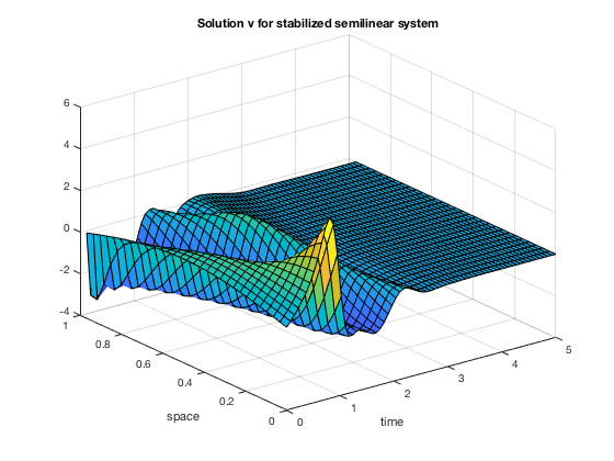
We compute the solution to the semilinear system with the same feedback control as the one found for the linear system:
F3 = @(t,z) A*z + B*f_ctr(z) + [z(1:n,1).*z(n+3:d,1);z(n+1, 1)*f_ctr(z);z(n+2, 1)^2 ; z(1:n,1).*z(n+3:d,1)];
[t3, Z3] = ode45(F3, time, z0);
The corresponding solutions $y$ and $v$ are displayed:
[X,Y] = meshgrid(t3, x1);
figure; surf(X, Y, Z3(:, 1:n+1)');
xlabel('time'); ylabel('space'); title('Solution y for stabilized semilinear system');

[X,Y] = meshgrid(t3, x2);
figure; surf(X, Y, Z3(:, n+2:2*(n+1))');
xlabel('time'); ylabel('space'); title('Solution v for stabilized semilinear system');
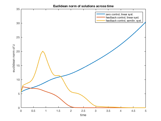
We compare the euclidean norm of the preceding solutions:
y1_norm = sum(abs(Z1(:, 1:n+1)).^2, 2);
y2_norm = sum(abs(Z2(:, 1:n+1)).^2, 2);
v1_norm = sum(abs(Z1(:, n+2:2*(n+1))).^2, 2);
v2_norm = sum(abs(Z2(:, n+2:2*(n+1))).^2, 2);
y3_norm = sum(abs(Z3(:, 1:n+1)).^2, 2);
v3_norm = sum(abs(Z3(:, n+2:2*(n+1))).^2, 2);
norm1 = (y1_norm + v1_norm).^(1/2);
norm2 = (y2_norm + v2_norm).^(1/2);
norm3 = (y3_norm + v3_norm).^(1/2);
figure;
plot(t1, norm1, 'lineWidth', 2);
hold on;
plot(t2, norm2, 'lineWidth', 2);
plot(t3, norm3, 'lineWidth', 2);
legend('zero control, linear syst.', 'feedback control, linear syst.', 'feedback control, semilin. syst.');
xlabel('time');
ylabel('euclidean norm of z');
title('Euclidean norm of solutions across time');
References
[1] Bastin G., J.-M. Coron, Stability and boundary stabilization of 1-D Hyperbolic systems. 2016.