Download Code
Model Problem
We consider the numerical approximation of the inverse problem for the linear advection-diffusion equation,
with $d$ being the diffusivity of the material and $v$ the direction of the advection.
Given a final time $T>0$ and a target function $u^\ast$ the aim is to identify the initial condition $u_0$ such that the solution, at time $t=T$, reaches the target $u^*$ or gets as close as possible to it. We assume that the initial condition $u_0$ is characterized as a combined set of sparse sources. This means that $u_0$ is a linear combination of unitary deltas with certain and possibly different weights, i.e:
We formulate the inverse problem using optimal control techniques. In particular, we consider the minimization of the following functional:
Space and time discretization
Letting $\textbf{u} : [0, T] \rightarrow \mathbb{R}^s$ where $s$ is the number of grid points on $\Omega$, we can write a general finite element (FE) discretization of the diffusion–advection equation in \eqref{modeleq} in a compact form as:
In order to get a time discretized version of the previous equation, we apply implicit Euler method with stepsize $\Delta t := T/N$ where $N$ is the total number of time steps. The numerical approximations to the solution are given by the vectors $\textbf{u}^n \approx \textbf{u}(t_n) \in \mathbb{R}^s$ with respect to the index $n=i\Delta t$ for $i=1,2,..,N$. Therefore, the fully discrete version of model equation is as follows,
Adjoint Algorithm for sparse source identification
The algorithm to be presented in this work for the sparse source identification of the linear diffusion-advection equation based on the adjoint methodology consists of two steps. Firstly, we use the adjoint methodology to identify the locations of the sources. Secondly, a least squares fitting is applied to find the corresponding intensities of the sources.
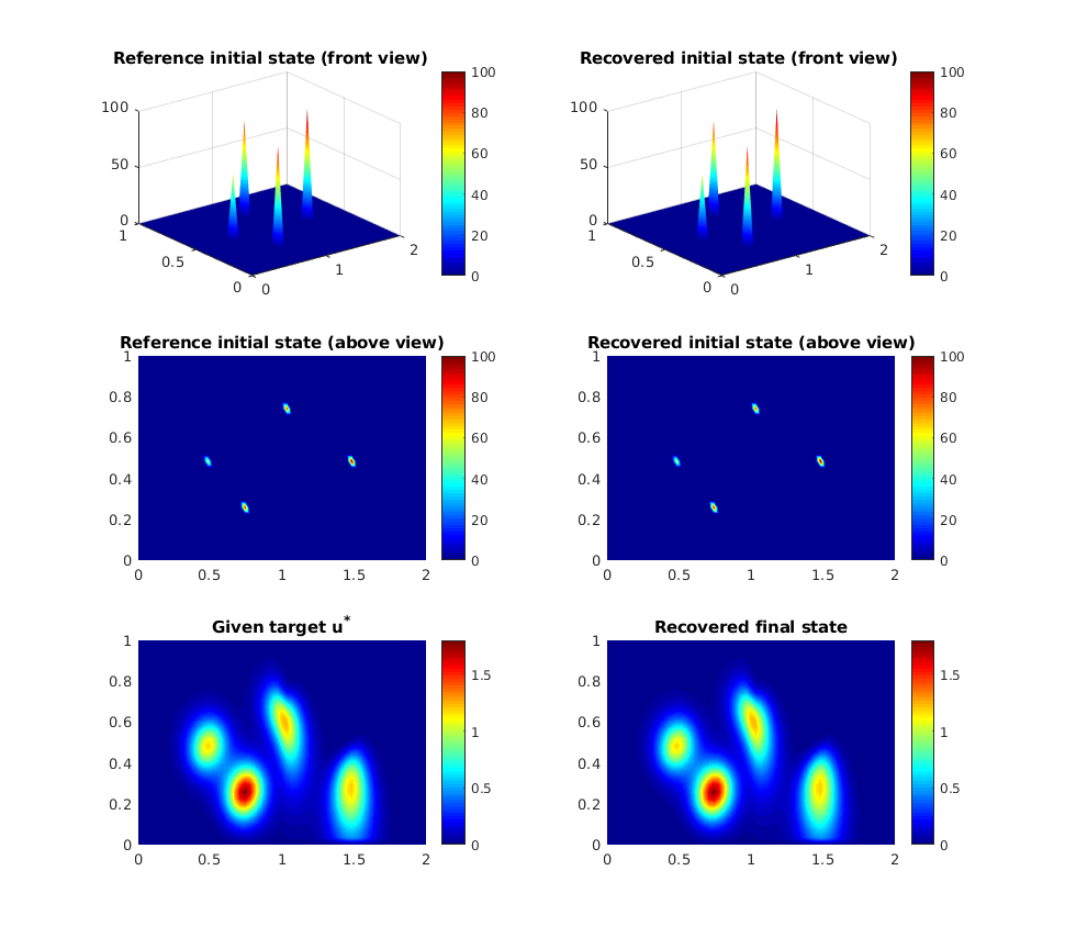
We have considered here a two-dimensional example with several sources to be identified in a multi-model environment. This means that the left half ($\Omega_1 = [0,1] \times [0,1]$) and the right half ($\Omega_2 = [1,2] \times [0,1]$) of the domain are modelled with different equations. In particular, the heat equation is used on $\Omega_1$ and the diffusion–advection equation is used on $\Omega_2$.
The initialization parameters look as follows:
N=30; %% space discretization points in y-direction
dx=1/(N+1); %% mesh size
t0=0; %% initial time
tf=0.1; %% final time
n=5; %% time discretization points
dt=(tf-t0)/n; %% stepsize
TOL=1e-5; %% stopping tolerance

d1=0.05; %% diffusivity of the material on the left sudomain
d2=0.05; %% diffusivity of the material on the left sudomain

%% advection components
vx=0;
vy=-3;

tau=dx^4; %% regularization parameter
epsilon=0.1; %% stepsize of the gradient descent method
We now compute the FE discretization matrices $M$, $A$ and $V$ that are respectively the mass matrix, the stiffness matrix and the advection matrix. For the FE discretization we assume equidistant structured meshes. In particular we use triangular elements and the classical pyramidal test functions are employed.
[M,A,V] = computeFEmatrices(N,d1,d2,vx,vy); %% Compute FE discretization matrices
A reference initial condition is chosen and we compute using the FE discretization specified above and implicit Euler in time its corresponding final state at time $T$. This final state will be considered the initial data of the inverse problem to be solved and we name it the target function $u^*$ as mentioned previously.
U0_ref = initial_deltas(N); %% computes reference initial condition

[U_target,u_target] = compute_target(U0_ref,N,n,dt,M,A,V); %% Compute target distribution
We now call the algorithm that estimates the initial condition $u_0$ using as a initial data the target function $u^*$. As mentioned before, this algorithm consists of two steps.
Firstly, the classical adjoint methodology that minimizes the functional $J(u_0)$ subject to the diffusion-advection equation is used. The iterative optimization algorithm employed is the classical gradient descent method. However, although this iterative procedure finds quite accurately the locations of the sources, it does not recover the sparse character of the initial condition. This is not suprising because the recovered initial data comes from solving the adjoint problem which is basically a diffusive process that smoothes out its state. Consequently, a second procedure is needed to project the obtained non sparse initial condition into the set of admissible sparse solutions.
As the initial condition $u_0$ is assumed to be a linear combination between the locations and the intensities, once we have fixed the locations using the adjoint methodology we can solve a least squares problem to get the remaining intensities. We assemble a matrix $\textbf{L} \in \mathbb{R}^{s \times l}$ where at each column we have the forward solution for a single unitary delta placed at each of the locations already identified. We then solve the following linear system of equations for the vector of unknowns $\alpha = (\alpha_1, \alpha_2, …, \alpha_l)^T$:
to find the intensities vector $\alpha$.
Adjoint algorithm for sparse source identification (algorithm 4)
U0 = SparseIdentification(u_target,TOL,dt,n,N,M,A,V,epsilon,tau);
Finally, the final state at $T$ is computed using as a initial condition the estimated sparse sources identified with our algorithm.
Compute final state with the recovered initial condition
[UF,u_final] = compute_target(U0,N,n,dt,M,A,V);
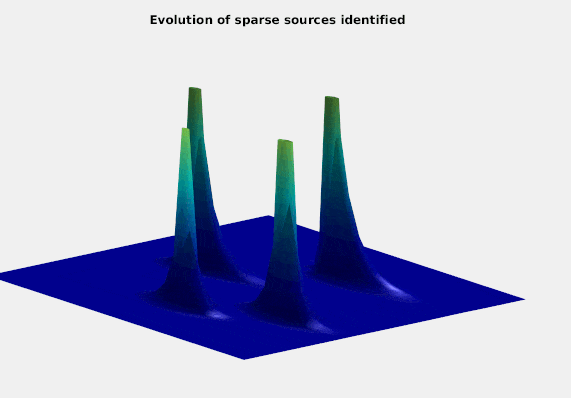
We can see the evolution recovered
We now visualize the numerical results. Plots on the left side show the reference initial solution and the given target. Similarly, plots on the right side show the recovered initial condition and the distribution at the final time $T$ produced by the recovered initial sources.
One can observe the difference between the two models (the heat equation on $\Omega_1$ and the diffusion-advection on $\Omega_2$) in the two figures at the bottom where the initial sources on $\Omega_2$ move downwards at the same time as they dissipate while the initial sources on $\Omega_1$ only dissipate without displacement.
xplot = linspace(0,2,2*N+3); %% space grid w.r.t component x
yplot = linspace(0,1,N+2); %% space grid w.r.t component y
%%
figure('unit','norm','pos',[0.25 0.1 0.5 0.8])
subplot(3,2,1)
surf(xplot,yplot,U0_ref)
shading interp;colorbar;colormap jet
title('Reference initial state (front view)')
subplot(3,2,2)
surf(xplot,yplot,U0)
shading interp;colorbar;colormap jet
title('Recovered initial state (front view)')
subplot(3,2,3)
pcolor(xplot,yplot,U0_ref)
shading interp;colorbar;colormap jet
title('Reference initial state (above view)')
subplot(3,2,4)
pcolor(xplot,yplot,U0)
shading interp;colorbar;colormap jet
title('Recovered initial state (above view)')
subplot(3,2,5)
pcolor(xplot,yplot,U_target)
shading interp;colorbar;colormap jet
title('Given target u^*')
subplot(3,2,6)
pcolor(xplot,yplot,UF)
shading interp;colorbar;colormap jet
title('Recovered final state')