Analysis, numerics and control for the obstacle problem

Download Code

In this tutorial, we present some aspects of the obstacle problem in the stationary (elliptic) and the evolutionary (parabolic) setting by means of numerical simulations, performed in FEniCS and Matlab.

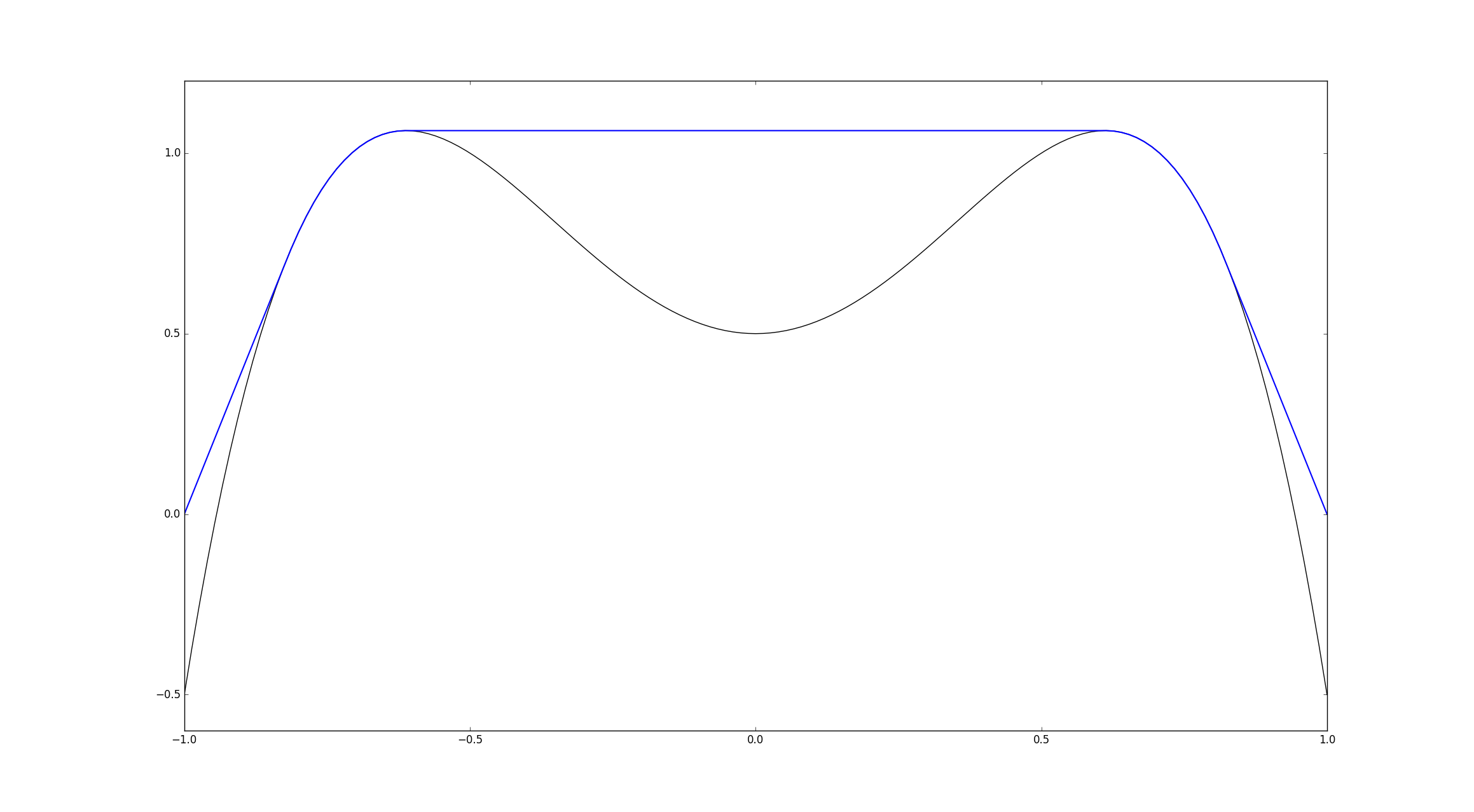Figure 1. The solution (blue) of the one-dimensional elliptic obstacle problem is superharmonic (concave down) and matches derivatives with the obstacle (black).

1. Mathematical formulation

1.1. Elliptic problem

Let $\Omega \subset \mathbb{R}^d$ be open, regular and bounded, let $\psi \in H^2(\Omega)$ (the obstacle) and $g \in H^1(\Omega)$ (boundary data) with $\psi \leq g$ on $\partial \Omega$ be given. We consider the functional

$\mathcal{F}_{\text{OB}}(u):= \frac12 \int_\Omega |\nabla u|^2 dx - \int_\Omega fu \, dx$

where $f \in L^2(\Omega)$ is given, and the closed convex set

$\mathcal{K}^g_{\text{OB}} := \{ u \in H^1(\Omega): u - g \in H^1_0(\Omega), \, u \geq \psi \, \text{ in } \, \Omega \}.$

The classical obstacle problem can be written as

$\min_{u \in \mathcal{K}^g_{\text{OB}}} \mathcal{F}_{\text{OB}}(u)$

and admits a unique minimizer $\phi \in \mathcal{K}^g_{\text{OB}}$, which is also a solution of the variational inequality

$\nabla \mathcal{F}_{\text{OB}}(\phi) \cdot (v-\phi) \geq 0 \quad \text{ for every } \quad v \in \mathcal{K}^g_{\text{OB}}.$

The terminology “obstacle problem” comes from the physical origin of the model $-$ the solution $\phi$ represents the equilibrium position of an elastic membrane, which is constrained to lie above an obstacle (given by the graph of the function $\psi$).

Notation: The notation

$\nabla \mathcal{F}_{\text{OB}}(\phi)\cdot\zeta$

designates the Gateaux derivative ($L^2$-gradient) of the functional ${F}_{\text{OB}}$ at the point $\phi$ in the direction $\zeta$; in occurence,

$\nabla \mathcal{F}_{\text{OB}}(\phi)\cdot\zeta = (\nabla \phi, \nabla \zeta)_{L^2(\Omega)}-(f, \zeta)_{L^2(\Omega)}-(g,\zeta)_{L^2(\partial \Omega)}$

Most of the regularity theory for the obstacle problem has been developed for the model case $\Delta \psi=-1$. We refer to [3,4] for a detailed presentation. For simplicity of the presentation, let us thus assume for a moment that $f \equiv -1$ and $\psi \equiv 0$. Choosing appropriate test functions bring us from the variational inequality for $\phi$ to

$\begin{cases} \Delta \phi = 1 &\text{ in } \{\phi>0\} \\ \phi \geq 0 &\text{ in } \Omega \\ \phi = |\nabla \phi| = 0 &\text{ on } \partial \{\phi>0\} \\ \phi = g &\text{ on } \partial \Omega. \end{cases}$

The set ${ \phi=0 }$ is called contact set, while $\partial { \phi>0 }$ is the free boundary.

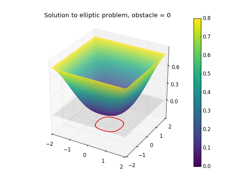Figure 2. The solution $\phi$ to the elliptic obstacle problem just above. The obstacle is equal to 0 (gray plane), and the free boundary (boundary of the contact set between the membrane and the obstacle) is displayed in red, projected just below.

Remark: At this point, we may see why solving the elliptic obstacle problem is different to just solving the Poisson equation for $\phi$ in a subdomain of $\Omega$ and setting $\phi=\psi$ elsewhere. Indeed, solving the latter problem does not guarantee that we would have

$|\nabla (\phi-\psi)| =0$

along the boundary.

1.2. Parabolic problem

The parabolic counterpart onsists in finding $u \in H^1(]0, +\infty[; L^2(\Omega))\cap L^2(]0,+\infty[; H^2(\Omega) \cap \mathcal{K}^g_{\text{OB}})$ satisfying

$\begin{cases} \big(\, u'(t), v-u(t) \big)_{L^2(\Omega)} + \nabla \mathcal{F}_{\text{OB}}(u(t))\cdot (v-u(t)) \geq 0 &\text{ for every } v \in \mathcal{K}^g_{\text{OB}}, \, t>0 \\ u(0, x) = u_0 \in \mathcal{K}^g_{\text{OB}}. \end{cases}$

The name “parabolic obstacle problem” for the above system may be misleading. While the mathematical formulation is similar, the physical interpretation of the elliptic and parabolic problem is different. In the parabolic setting, seeing $\psi$ as a physical obstacle in space is not correct. Rather, one should interpret $\psi$ as a barrier for the temperature $u$. More accurately, we are dealing with a parabolic variational inequality with an obstacle-type constraint.

The function $\psi$ may be time-dependent, but for simplicity we omit this case.

Figure 3. Here $\psi(x)=3*\sqrt{(1-x^2)}$ in $(-1,1)$ (black) is a barrier for the evolving solution (blue). The initial data coincides with $\psi$ on (-1.5, 1.5). We observe that the contact set $\{ u = \psi \}$ changes (gets smaller) as time grows. There is also matching of normal derivatives on the contact points (i.e. the free boundary). Finally, the solution of the parabolic problem (left, blue) converges to that of the elliptic problem (right, red) for large time, as seen below.

Figure 4. The solution to the parabolic problem with Dirichlet boundary condition =1. The obstacle is given by the "three towers". The free boundary (boundary of the contact set with the obstacle) is projected on a plane below in red. It is seen that the source term $-1$ acts as a gravity force pushing the membrane towards the obstacle. We moreover observe a convergence to the equilibrium position (see also the section below).

For $\psi \equiv 0$ and $f\equiv-1$ (or more generally $f + \Delta \psi = -1$), a manifestation of the parabolic variational inequality above is as a “weak form” of the one-phase Stefan problem (see [3,4]). In this setting, we may pass from the variational inequality to the equivalent problem with two boundary conditions at the free boundary

$\begin{cases} u_t - \Delta u = -1 &\text{ in } \quad \{ u(t)>0\} \times ]0, +\infty[ \\ u \geq 0 &\text{ in } \quad \Omega \times ]0, +\infty[ \\ u = |\nabla u| = 0 &\text{ on } \quad \partial \{ u(t)>0 \} \times ]0, +\infty[\\ u = g &\text{ on } \quad \partial \Omega \times ]0, +\infty[ \\ u = u_0 &\text{ on } \quad \Omega \times \{ t = 0\} \end{cases}$

This is an overdetermined problem, which means that the free boundary/the contact set ${u=0}$ has to change with time to ensure that both BC hold for every time. The evolution of the contact set may be observed in the numerics of Figures 3,4,5.

Remark: $\quad$ As for the elliptic problem, solving the above parabolic problem is different to just solving the heat equation for $u$ in a subdomain of $\Omega$ and setting $u$ elsewhere, with a Dirichlet boundary condition. Indeed, solving the latter problem does not guarantee that we would have $|\nabla u|= 0$ along the boundary.

Remark: $\quad$ While in Figure 3 the contact set is shrinking does not disappear, it may happen that the contact set vanishes (depending on the magnitude of the boundary data $g$, the support of the initial data $u_0$, and if present, the source term $f$).

1.3. Relationship between both problems

In the recent paper [5], it is shown that the solution $u(t)$ to the parabolic variational inequality converges to the solution $\phi$ of the elliptic probelem in $H^1(\Omega)$ norm as $t\rightarrow \infty$ with exponential rate. This is done by means of new techniques including a so-called constrained Lojaseiwicz inequality.

We may observe this convergence numerically in Figures 4 and 5. In both cases, we work in the ball $B_2$, with boundary data $g\equiv 0.8$, barrier $\psi\equiv 0$ and initial datum supported outside $B_{1.5}$.

The one-dimensional case:

Figure 5. The solution of the parabolic problem (left, blue) converges to that of the elliptic problem (right, red) as time increases. We again see that the contact set $\{ u = 0\}$ changes with time.

The two-dimensional case:

Figure 6. We see that as time increases, the contact region $\{ u = 0\}$ (white patch) gets smaller. In terms of the Stefan problem, the white patch represents the ice temperature. Ice is melting as time increases, but does not fully melt, because the support of the initial data is too small and the temperature on the boundary is not high enough.

Figure 7. In this figure, the obstacle is set to zero, and we consider Dirichlet boundary conditions $=0.8$ on the fixed boundary. We see that even when considering initial data which are not an equilibrum membrane position (but do satisfy the obstacle condition), as time increases, the solution of the parabolic problem (left) converges to that of the elliptic problem (right)

2. Numerical implementation

2.1. Possible strategies

A common approach for proving the well-posedness and $W^{2,p}$ regularity for variational inequalities is a technique called penalization, which consists of approximating by a sequence of semilinear equations [8]. For any $\epsilon>0$, we will consider

$u' - \Delta u + \frac{1}{\epsilon} (u-\psi)_{-} = f \quad \text{ in } \quad \Omega \times ]0,\infty[$

to approximate the parabolic problem, and remove $u’$ and time dependence for the elliptic one. As $\epsilon\rightarrow0$, the solution $u_\epsilon$ of the above equation converges to the variational inequality. Here

$\beta_\epsilon(u) = \frac{1}{\epsilon}(u)_- = \frac{1}{\epsilon}\min \{u, 0 \}$

may be replaced by another penalty function, for instance $\beta_\epsilon(u) = -\exp(-u/\epsilon)$.

The approximated problem is relatively simple to implement numerically. We may use finite elements (say $P1$ elements) to discretize in space, and time-stepping (Euler implicit for instance) to discretize in time.

There are other ways to solve the variational inequality after discretizing in space and time (using one’s favorite metood). One which is popular in the literature for the elliptic problem is the primal dual active set method, which we will present in a future post.

2.2. Code

i). Elliptic problem.

Let us start by solving the two-dimensional elliptic problem from Figure 4.

The fenics module [1] contains all of the necessary finite element tools for the space discretization of PDEs.

from fenics import *
from obstacles import dome
from mshr import mesh

It is advantageous to regularize the “kink” appearing in penalty function (the negative part of a function) in view of using a Newton method for solving the nonlinear problem

def smoothmax(r, eps=1e-4): 
	return conditional(gt(r, eps), r-eps/2, conditional(lt(r, 0), 0, r**2/(2*eps)))

We mesh the domain $B_2$.

mesh = generate_mesh(Circle(Point(0, 0), 2), 25)

$P1$ elements are used for the FEM spaces (but one may easily choose higher order in the definition of V).

V = FunctionSpace(mesh, "CG", 1)
w = Function(V)
v = TestFunction(V)
psi = Constant(0.)
f = Constant(-1)		
eps = Constant(pow(10, -8))

Using the symbolic expressions of FEniCS, we define the variational formulation of the penalized PDE, which we write in the form $F(w)=0$:

bc = DirichletBC(V, 0.8, "on_boundary")
F = dot(grad(w), grad(v))*dx - 1/eps*inner(smoothmax(-w+psi), v)*dx - f*v*dx

We solve the nonliner problem with the command solve, which makes use of a Newton method to solve the nonlinear equation $F(w)=0$.

solve(F == 0, w, bcs=bc)

We visualise in ParaView by storing the solution in .vtk format using:

vtkel = File("output/el.pvd")
vtkel << w

ii). Parabolic problem.

We set $T=2$, use $100$ subdivisions and set

dt = T/100

This part only differs by the presence of a time-loop. We define the initial datum in a separate class:

class indata(Expression):
	def eval(self, value, x):
		if sqrt(x[0]*x[0]+x[1]*x[1]) <= 1.95:
			value[0] = 0
		elif 1.95 <= sqrt(x[0]*x[0] + x[1]*x[1]) <= 2:
			value[0] = (sqrt(x[0]*x[0]+x[1]*x[1])-1.95)/(2-1.95)*0.8
		else:
			value[0] = 0.8

Repeating as in the elliptic case up to defining the variational form, we now set the inital datum (interpolating the expression onto the FEM space) and time:

un = interpolate(indata(degree=2), V)
t = 0

We set up the time loop:

vtksol = File("output/popsol.pvd")
for n in range(num_steps):
    t+=dt
    solve(F==0, u, bcs=bc)
    vtksol << (u, t)
    un.assign(u)

Optimal Control

We will now briefly present the implementation of an optimal control strategy for the elliptic and parabolic problems. We will make use of the penalized problems where $\epsilon>0$ is small (of the order $10^{-8}$). This strategy has been succesfully applied in [8].

3.1. Elliptic problem

Given a target $\phi_d$ and a regularization parameter $\delta>0$ (we usually use $\delta = 10^{-2}$), we seek to minimize

$J(u) = \frac12 \|\phi-\phi_d \|_{L^2(\Omega)}^2 + \frac{\delta}{2} \| u \|^2_{L^2(\Omega)}$

subject to

$\begin{cases} -\Delta \phi + \frac{1}{\epsilon} (\phi-\psi)_- = f+u &\text{ in } \Omega \\ \phi = g &\text{ on } \partial \Omega. \end{cases}$

For simplicity of the presentation, we will consider

$f\equiv-1$ $g\equiv0\$ $\psi(x) = \sqrt{(1-|x|^2)_+}$

on the domain $\Omega = [-2,2]^2$. The target is the function $\phi_d(x) = \frac12(\cos(x_1)+\cos(x_2))$.

The uncontrolled solution of the elliptic obstacle problem in this case is:

Figure 8. For comparison with the controlled problem, we show also the solution to the free elliptic problem with the "dome" like obstacle given on the right.

The FEniCS optimization code will have the effect of obtaining the following results.

Figure 9. The optimal state (top left) can be seen to be above the obstacle (top right), and is very much alike the shape of the target (bottom left). Finally, the optimal control is given (bottom right).

Let us present the numerical implementation. After importing the dolfin_adjoint optimization module [2], we make use of the code for simulating the uncontrolled problem. A “tape” of the forward model is built. This tape is used to drive the optimization by repeatedly solving the forward model and the adjoint model for varying control inputs.

Defining the objective functional to be minimized:

delta = Constant(1e-2)
j = assemble(0.5*inner(w-wd, w-wd)*dx + delta/2*inner(u, u)*dx)	
m = Control(u)

Writing the state $y$ as the output of the solution map corresponding to the input $m$, one sees that the objective functional depends only on the control:

J = ReducedFunctional(j, m)

We run the optimization, based on a conjugate-gradient method:

u_opt = minimize(J, options={"method"="CG"})

The tape is modified such that the initial guess for y (to be used in the Newton solver in the forward problem) is set to y_opt.

y_opt = y.block_variable.saved_output
Control(y).update(y_opt)

The algorithm converged after 8 iterations, and the value of the functional at the final iteration is $0.0967$.

3.2. The parabolic problem

Given a final time $T>0$, a target $u_d$ and a regularization parameter $\delta>0$, we seek to minimize

$J(u) = \frac12 \|u(T)-u_d \|_{L^2(\Omega)}^2 + \frac{\delta}{2} \| v \|_{L^2(\Omega)}$

subject to

$\begin{cases} u'-\Delta u + \frac{1}{\epsilon} (u)_- = f+v &\text{ in } \Omega \times (0, T) \\ u = g &\text{ on } \partial \Omega \times (0, T) \\ u = u_0 &\text{ in } \Omega \times \{ t = 0 \} \end{cases}$

For simplicity of the presentation, we will consider the same setting as in Figure 3, namely $f\equiv-1\,$, $g\equiv0.8\,$, on the domain $\Omega = [-2,2]$. The target temperature is $u_d(x) = 0.8$. This would correspond to “melting”, as this target is never equal to zero, thus has no contact set. We would thus expect the action of the control $v$ to lift-up $u$ from $0$ and thus the contact set (and free boundary) to vanish.

We appeal to DyCon-Toolbox [9] for the numerical implementation of this problem. DyCon-Toolbox is an efficient and easy to use solver for nonlinear control problems.

Figure 10. The optimal state (left, red), starting from an initial datum with a non-empty contact set (left, blue) and the optimal control (red, right).

The action and magnitude of the control ensures that the solution to the parabolic problem will lift-off from the initial contact set. For comparison, we recall that the uncontroled free dynamics have a very different behavior:

Figure 11. The uncontrolled free dynamics of the parabolic obstacle problem in 1 dimension, where the obstacle is zero.

We begin by symbolically defining the time variable:

syms t

We discretize the interval $[-2, 2]$:

N = 70;
xi = -2; xf = 2;
xline = linspace(xi,xf,N+2);
xline = xline(2:end-1);

We define symbolically (as in FEniCS) the state vector $Y$ and control vector $U$:

Y = SymsVector('y',N);
U = SymsVector('u',N);

We discretize by finite differences, and define the semilinear penalty term:

alpha = 1e-3;
epsilon = 1e-2;
A = FDLaplacian(xline);

F  = @(Y) NonLinearTerm(Y,alpha);
dF = @(Y) DiffNonLinearTerm(Y,alpha);

We may define the parabolic problem to be solved.

dx = xline(2) - xline(1);
Y_t = @(t,Y,U,Params) A*Y + 1/epsilon*F(-Y) + U + (1/dx^2)*[0.8;zeros(N-2,1);0.8];
Dyn = pde(Y_t,Y,U);

We set the mesh, and other relevant parameters such as the final time and initial data. We consider the same data as in the free problem.

Dyn.mesh   = xline;
Dyn.Solver = @ode23;
Dyn.Nt     = 150;
Dyn.FinalTime        = 0.3;
Dyn.InitialCondition = InitialConditionFcn(xline);

We now compute the necessary Jacobian matrices.

Dyn.Derivatives.Control.Num = @(t,Y,U,Params) eye(N);
Dyn.Derivatives.State.Num   = @(t,Y,U,Params) A + 1/epsilon*dF(-Y);

We may solve the free problem over the given time interval. We recall that we have used finite differences to discretize in space (but finite elements can be used as well in more complicated settings), and the underlying solve command solves the system of ODEs by means of some Runge-Kutta scheme.

[tspan,Ysolution] = solve(Dyn);
figure
surf(Ysolution)

Having solved the free dynamics, we are now in a position to solve the optimal control problem:

YT = 0.8 + 0*xline';
beta = dx^4;
Psi  = @(T,Y) dx*(YT - Y).'*(YT - Y);
L    = @(t,Y,U)  dx*(YT - Y).'*(YT - Y) + ...
                 beta*dx*0.5*alpha*(U.'*U);
OCP = Pontryagin(Dyn,Psi,L);
U0 = -ones(Dyn.Nt,Dyn.ControlDimension);
U0 = GradientMethod(OCP,U0,'Graphs',true,'EachIter',2,'DescentAlgorithm',@AdaptativeDescent)

References:

[1] The FEniCS Project Version 1.5 M. S. Alnaes, J. Blechta, J. Hake, A. Johansson, B. Kehlet, A. Logg, C. Richardson, J. Ring, M. E. Rognes and G. N. Wells Archive of Numerical Software, vol. 3, 2015.

[2] Patrick E. Farrell, David A. Ham, Simon W. Funke and Marie E. Rognes (2013). Automated derivation of the adjoint of high-level transient finite element programs, SIAM Journal on Scientific Computing 35.4, pp. C369-C393. doi:10.1137/120873558. arXiv:1204.5577

[3] Figalli A. (2018), Free boundary regularity in obstacle problems Journées EDP 2018, to appear.

[4] Figalli, A. (2018), Regularity of interfaces in phase transitions via obstacle problems Proceedings ICM 2018, to appear.

[5] Colombo M. and Spolaor, L. and Velichkov, B. (2018), On the asymptotic behavior of the solutions to parabolic variational inequalities, ArXiV preprint.

[6] Borjan Geshkovski (2018). Obstacle Problems: Theory and Applications. Master Thesis.

[7] Hintermüller M. and Kopacka I., A smooth penalty approach and a nonlinear multigrid algorithm for elliptic MPECs. Computational Optimization and Applications, 50(1):111–145, 2011.

[8] D. Kinderlehrer and G. Stampacchia. An introduction to variational inequalities and their applications. Volume 31 of Classics in Applied Mathematics. SIAM, 2000.

[9] DyCon-Toolbox, https://deustotech.github.io/dycon-toolbox-documentation/.

Work Packages ≻ Control under constraints ≻