Download Code
Control of reaction-diffusion
This is a post in a collection of several on control of reaction-diffusion under state constraints
See more ...
This tutorial is focused on the understanding of of the problem
The solutions for $a=0$ constitute an intrinsic obstruction to the controllability with state-constraints due to the comparison principle [1]. Indeed, for any control function $0\leq a(x,t)\leq 1$
the solution of the problem:
where $u$ is an elliptic nontrivial solution satisfies that $v(x,t)\geq u(x)$. Therefore, we cannot expect to control to any function below $u$.
This is why the understanding of the existence or non-existence of nontrivial solutions is of main importance for the controllability under state-constraints.
Non-trivial solutions around the boundary value $a=\theta$ do not constitute an intrinsic obstruction to the controllability because the boundary value $\theta$ is not in the border of the admissible set. However, the existence of such solutions create a technical difficulty for achieving the controllability to the steady state $w\equiv \theta$ which can be solved by constructing paths of steady states (See this blog entry ).
Elliptic nontrivial solutions with boundary value 1 do not exist. This can be related to the fact that the traveling waves for the Cauchy problem in the real line are approaching the steady state $w\equiv 1$ [2]
The existence of non-trivial solutions can be done either by comparison principles or by understanding the critical points of a functional (see [3]).
Any critical point of the functional:
is a weak solution of the main equation.
In order to guarantee that the solution will be between $0$ and $1$, one can extend $f$ by $0$ outside of the interval $[0,1]$.
Restricting ourselves in the one dimensional case (the argument also holds in several dimensions) and making the spatial change fo variables $x\to \frac{x}{L}$, where $L$ is the length of the domain the functional reads:
In the expression above we see that if $L$ is small the convex part dominates while if $L$ is large and $\int_0^1f(s)ds>0$ it might not be convex.
In the videos below one can see the evolution of the functional depending on the parameter $\lambda=L^2$. The representation is the evaluation of the functional along the first and the third eigenfunction, i.e. $e_1=\sin(\pi x)$ and $e_3=\sin(3\pi x)$,
Here, one can see the evolution of the functional for $a=0$ and for $a=\theta=1/3$ for values of $\alpha$ and $\beta$.
Figure 1. Animation of the functional $J$ for diferent values of $\lambda=L^2$. At the left the boundary value is $0$ while at the right the boundary value is $\theta$.
In the next figure a qualitative bifurcation diagram is represented, the red curve represents the nontrivial solutions with boundary value $\theta$ and the blue one the boundary value $0$. $\lambda^\ast$ is the minimum $\lambda=L^2$ for which a nontrivial solution around $0$ exists, analogously $\lambda^*_\theta$.
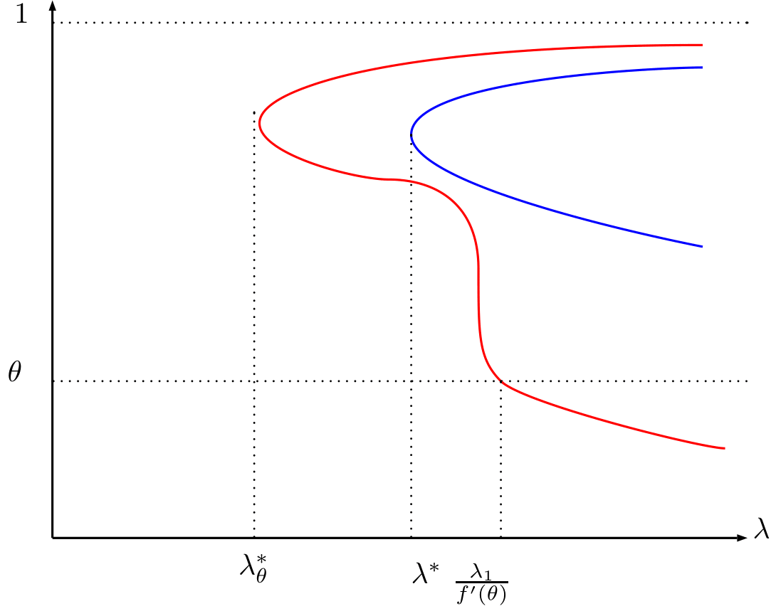 Figure 2. Bifurcation diagram . The blue line represents the maximum of the nontrivial solutions with boundary value $0$. The red curve represents some nontrivial solutions with boundary value $\theta$, the red line is the maximum of the nontrivial solution whenever the line is above $\theta$ and represents the minimum when the red line is below $\theta$.
The value $\frac{\lambda_1}{f’(\theta)}$ is the critical value for which the stationary solution $\theta$ becomes unstable. After this situation we have a nontrivial solution above and below $\theta$.
There will be further bifurcations around the boundary value $\theta$ when we increase $\lambda$. These bifuractions will lead to oscillatory nontrivial solutions that can be well understood in the phase-plane, see [2].
Here one can see different non-trivial solutions for different boundary values. The green curve corresponds to a section of the nontrivial solution in the whole $\mathbb{R}$:
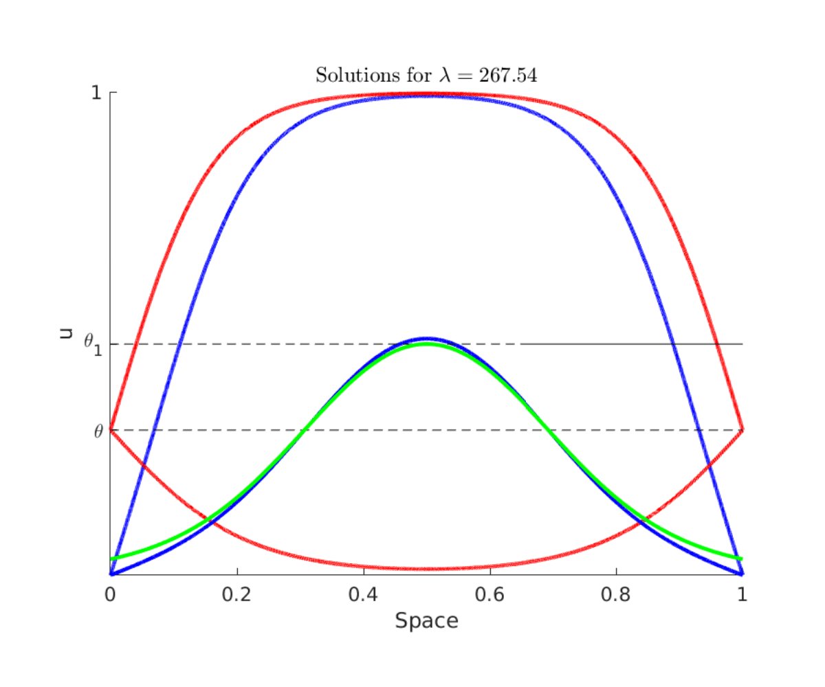 Figure 3. Several nontrivial solutions, in blue the ones with boundary value $0$, the red ones have boundary value $\theta$ and the green one is the solution in the whole $\mathbb{R}$. $\theta_1$ is the number such that $\int_0^{\theta_1} f(s)ds = 0 $.
References:
[1] M.H. Protter and H.F. Weinberger, Maximum principles in differential equations, Springer Science & Business Media, 2012.
[2] D. Ruiz-Balet and E. Zuazua. Control of certain parabolic models from biology and social sciences. Preprint available at https://cmc.deusto.eus/domenec-ruiz-balet/.
[3] P.L. Lions, On the existence of positive solutions of semilinear elliptic equations, SIAM Rev. 24 (1982), no. 4, 441–467.