Download Code
Control of reaction-diffusion
This is a post in a collection of several on control of reaction-diffusion under state constraints
See more ...
Equation and drift effect
The equation under concern is:
where $N$ is a positive regular function.
The physical meaning of the equation is a reaction-diffusion process on the proportion $u$ of individuals along a static heterogeneous distribution $N$.
The effect of this heterogeneous drift can be qualitatively understood in Figure 1. The blue line in the figure is the distribution $N$ and the orange one the term $-2\frac{N_x}{N}$. In the picture in the left we have the Gaussian with variance $\sigma$, leading to a drift effect that is pushing $u$ towards the boundary. At the right, we have the function $e^{x^2/\sigma}$ leading to the contrary effect, the population in the boundary is pushed inside the domain.
From the discussion above we expect the boundary control to be enhanced in the case of $N(x)=e^{x^2/\sigma}$ while diminished in the case of $N(x)=e^{-x^2/\sigma}$.
Figure 1. In blue the curves $N(x)=e^{\mp x^2/\sigma}$ and in orange the term $-2\frac{N_x}{N}$.
Slowly varying drifts: Perturbed Stair-case method
Whenever the drift term $-2\frac{N_x}{N}$ is small enough, one can consider the already developed path in the homogeneous setting (see Blog staircaise), taka a sequence and apply the implicit function theorem to obtain a sequence close enough to guarantee the controllability (see [1] for details). This guarantees the controllability from the steady state $0$ to the target $\theta$.
In Figure 2 an intuitive sketch of this procedure is represented.
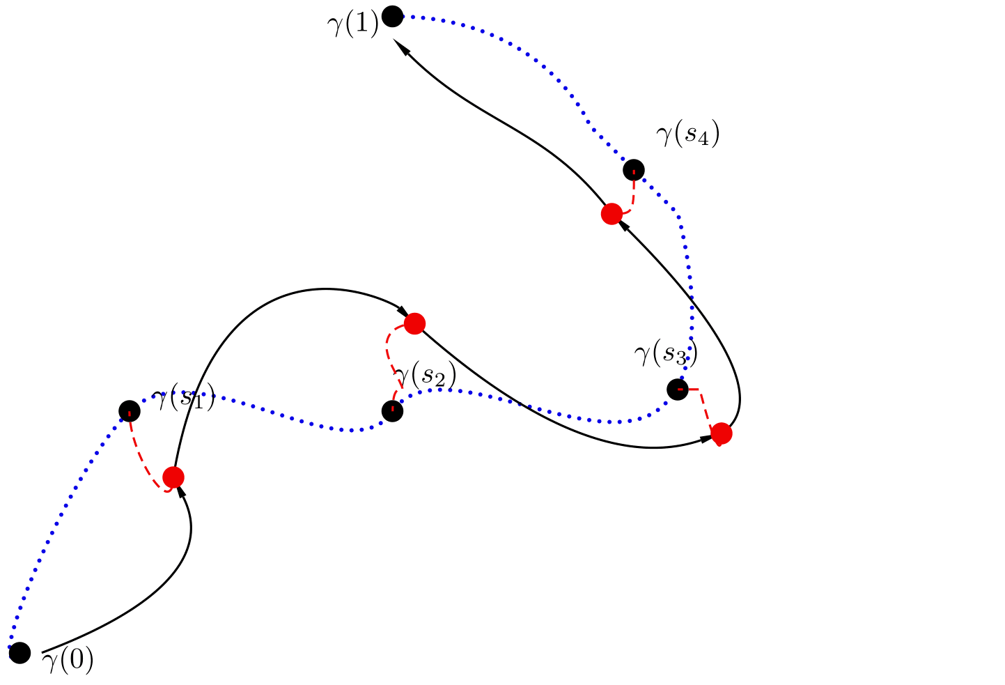 Figure 2. Perturbed staircase method.
Large drifts: New Barriers
One of the main concerns when state-constraints are present is whether or not barriers exist (see Blog Barriers). If $\theta<\frac{1}{2}$ then, for large $L>L_{\sigma}(0)>0$ we will have obstructions to reach $\theta$ and $0$ from $1$.
In the homogeneous case, nontrivial elliptic solutions with boundary value $1$ do not exist. However, in the case of heterogeneous drift this is no longer true in general.
If we set $N(x)=e^{-x^2/\sigma}$ then for every $\sigma$ one can find an $L_{\sigma}(1)>0$ big enough such that for every $L>L_{\sigma}$ there is a nontrivial solution with boundary value $1$. This nontrivial solution does not correspond to a global minima of the associated energy functional since the trivial solution $u=1$ is the global minimizer.
In order to understand how this barrier can exist we have to study the following non-autonomous dynamics in the phase-plane:
Any solution of the ODE above is an elliptic solution for some boundary condition. What we want to find is that there exist an $L_{\sigma}(1)$ such that the solution of the ODE at $L_{\sigma}(1)$ is $1$.
Making use of the energy of the ODE
and seting $a$ small one can see that the trajectory of the dynamics will eventually cross $1$. See Figure 3.
Figure 3. At the left, the trajectory in the phase-plane associated with the elliptic solution. At the right, the resulting nontrivial solution.
In Figure 4 one can see the effect of the nontrivial solution in a simulation. The red lines are snapshots of the controlled trajectory, getting darker when advancing the time, the dotted blue line is the profile $N(x)$.
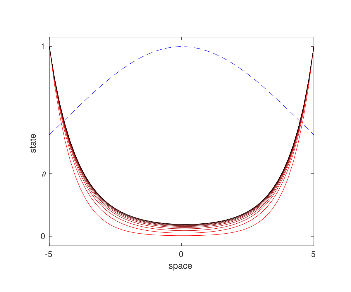 Figure 4. Simulation of the equation with control $a=1$ with $N(x)=e^{-x^2/\sigma}$.
Minimal controllability time depending on the drift
We have seen that the influence of the drift is key. Figure 5 shows the minimal controllability time for a fixed $L$ depending on the parameter $\frac{1}{\sigma}$. The initial state is the $0$ configuration and the target the constant steady state $\theta$.
When the variance is very big we tend to the homogeneous case, while when the variance decreases the opposite phenomena is observed; when the drift enhances the control the minimal controllability time is reduced making it tend to zero while, when the drift is pushing the population outside the minimal controllability time increases and eventually blows up with the emergence of the barrier.
Figure 5. Minimal controllability time depending on the variance. At the left for $N(x)=e^{x^2/\sigma}$ and at the right for $N(x)=e^{-x^2/\sigma}$.
References:
[1] I. Mazari, D. Ruiz-Balet, and E. Zuazua, Constrained control of bistable reaction-diffusion equations: Gene-flow and spatially heterogeneous models, preprint: https://hal.archives-ouvertes.fr/hal-02373668/document (2019).
[2] D. Pighin, E. Zuazua, Controllability under positivity constraints of multi-d wave equations, in:
Trends in Control Theory and Partial Differential Equations, Springer, 2019, pp. 195–232.
[3] J.-M. Coron, E. Trélat, Global steady-state controllability of one-dimensional semilinear heat equa-
tions, SIAM J. Control. Optim. 43 (2) (2004) 549–569.
[4] C. Pouchol, E. Trélat, E. Zuazua, Phase portrait control for 1d monostable and bistable reac-
635
tion–diffusion equations, Nonlinearity 32 (3) (2019) 884–909.
[5] D. Ruiz-Balet and E. Zuazua. Controllability under constraints for reaction-diffusionequations: The multi-dimensional case. Preprint available athttps://cmc.deusto.eus/domenec-ruiz-balet/.
[6] D. Ruiz-Balet and E. Zuazua. Control of certain parabolic models from biology and social sciences. Preprint available at https://cmc.deusto.eus/domenec-ruiz-balet/.