Download Code
In this tutorial, we present how to use Pontryagin environment to control a consensus system that models the complex emergent dynamics over a given network. The control basically minimize the cost functional which contains the running cost and desired final state.
Setup
In this tutorial we need DyCon Toolbox, to install it we will have to write the following in our MATLAB console:
unzip('https://github.com/DeustoTech/DyCon-Computational-Platform/archive/master.zip')
addpath(genpath(fullfile(cd,'DyCon-toolbox-master')))
StartDyConToolbox
You can see the code of this tutorial write the following line:
open T06ODET0004_Kuramoto
Model
The Kuramoto model describes the phases $\theta_i$ of active oscillators, which is described by the following dynamics:
Here, the first constant terms $\omega_i$ denote the natural oscillatory behaviors, and the interactions are nonlinearly affected by the relative phases. The amplitude and connections of interactions are determined by the coupling strength, $K_{i,j}$.
Control strategy
The control interface is on the coupling strength as follows:
This is a nonlinear version of bi-linear control problem for the Kuramoto interactions. The idea is as follows;
-
There are $N$ number of oscillators, oscillating with their own natural frequencies.
-
We want to make a collective behavior using their own decision process. The interaction is given by the Kuramoto model, or may follow other interaction rules. The network can be given or flexible with control.
-
The cost of control will be related to the collective dynamics we want, such as the variance of frequencies or phases.
Numerical simulation
Here, we consider a simple problem: we control the all-to-all network system to get gathered phases at final time $T$. We first need to define the system of ODEs in terms of symbolic variables.
clear all
m = 50;  %% [m]: number of oscillators.

import casadi.*

t     = SX.sym('t');
symTh = SX.sym('y', [m,1]);   %% [y] :  phases of oscillators, $\theta_i$.
symOm = SX.sym('om', [m,1]);  %% [om]:  natural frequencies of osc., $\omega_i$.
symK  = SX.sym('K',[m,m]);    %% [K] :  the coupling network matrix, $K_{i,j}$.
symU  = SX.sym('u',[1,1]);    %% [u] :  the control function along time, $u(t)$.


syms Vsys;    %% [Vsys]: the vector fields of ODEs.
symThth = repmat(symTh,[1 m]);
Vsys = casadi.Function('V',{symOm,symK,symTh,symU}, ...
{ symOm + (symU./m)*sum(symK.*sin(repmat(symTh,[1 m]).' - repmat(symTh,[1 m])),2) });
The parameter $\omega_i$ and $K_{i,j}$ should be specified for the calculations. Practically, $K_{i,j}u(t) > \vert \max\Omega - \min\Omega \vert$ leads to the synchronization of frequencies. We normalize the coupling strength to 1, and give random values for the natural frequencies from the normal distribution $N(0,0.1)$. We also choose initial data from $N(0,\pi/4)$.
rng('default');
rng(1,'twister');
Om_init = normrnd(0,0.2,m,1);
Om_init = Om_init - mean(Om_init);  %% Mean zero frequencies
Th_init = normrnd(0,pi/8,m,1);
K_init = ones(m,m);                 %% Constant coupling strength, 1.
T = 5;                              %% We give enough time for the frequency synchronization.
symF = casadi.Function('F',{t,symTh,symU},{Vsys(Om_init,K_init,symTh,symU)});

tspan = linspace(0,T,110);
odeEqn = ode(symF,symTh,symU,tspan);
SetIntegrator(odeEqn,'RK4')
odeEqn.InitialCondition = Th_init;
We next construct cost functional for the control problem.
PathCost  = casadi.Function('L'  ,{t,symTh,symU},{ (1/2)*(symU'*symU)           });
FinalCost = casadi.Function('Psi',{symTh}      ,{  1e5*(1/m^2)*sum(sum((symThth.' - symThth).^2))  });

iCP_1 = ocp(odeEqn,PathCost,FinalCost);
Solve Gradient descent
tic
ControlGuess = ZerosControl(odeEqn);
[OptControl_1 ,OptThetaVector_1] =  ArmijoGradient(iCP_1,ControlGuess);
toc
Length Step has been change: LenghtStep = 0.00025
iter: 001 | error: 2.215e+02 | LengthStep: 5.00e-04 | J: 1.16893e+03 | Distance2Target: NaN
iter: 002 | error: 2.214e+02 | LengthStep: 1.00e-03 | J: 1.16780e+03 | Distance2Target: NaN
iter: 003 | error: 2.212e+02 | LengthStep: 2.00e-03 | J: 1.16554e+03 | Distance2Target: NaN
iter: 004 | error: 2.207e+02 | LengthStep: 4.00e-03 | J: 1.16103e+03 | Distance2Target: NaN
iter: 005 | error: 2.198e+02 | LengthStep: 8.00e-03 | J: 1.15206e+03 | Distance2Target: NaN
iter: 006 | error: 2.180e+02 | LengthStep: 1.60e-02 | J: 1.13430e+03 | Distance2Target: NaN
iter: 007 | error: 2.144e+02 | LengthStep: 3.20e-02 | J: 1.09950e+03 | Distance2Target: NaN
iter: 008 | error: 2.074e+02 | LengthStep: 6.40e-02 | J: 1.03270e+03 | Distance2Target: NaN
iter: 009 | error: 1.938e+02 | LengthStep: 1.28e-01 | J: 9.09692e+02 | Distance2Target: NaN
iter: 010 | error: 1.682e+02 | LengthStep: 2.56e-01 | J: 7.01968e+02 | Distance2Target: NaN
iter: 011 | error: 1.235e+02 | LengthStep: 5.12e-01 | J: 4.10547e+02 | Distance2Target: NaN
iter: 012 | error: 6.257e+01 | LengthStep: 1.02e+00 | J: 1.47399e+02 | Distance2Target: NaN
Length Step has been change: LenghtStep = 0.256
iter: 013 | error: 4.113e+01 | LengthStep: 5.12e-01 | J: 1.20852e+02 | Distance2Target: NaN
iter: 014 | error: 2.215e+01 | LengthStep: 1.02e+00 | J: 9.58348e+01 | Distance2Target: NaN
Length Step has been change: LenghtStep = 0.256
Length Step has been change: LenghtStep = 0.064
Length Step has been change: LenghtStep = 0.016
Length Step has been change: LenghtStep = 0.004
Length Step has been change: LenghtStep = 0.001
Length Step has been change: LenghtStep = 0.00025
Length Step has been change: LenghtStep = 6.25e-05
Length Step has been change: LenghtStep = 1.5625e-05
Length Step has been change: LenghtStep = 3.9063e-06
Length Step has been change: LenghtStep = 9.7656e-07
Length Step has been change: LenghtStep = 2.4414e-07
Length Step has been change: LenghtStep = 6.1035e-08
Length Step has been change: LenghtStep = 1.5259e-08
Length Step has been change: LenghtStep = 3.8147e-09

    Mininum Length Step have been achive !!

Elapsed time is 2.131655 seconds.
Visualization
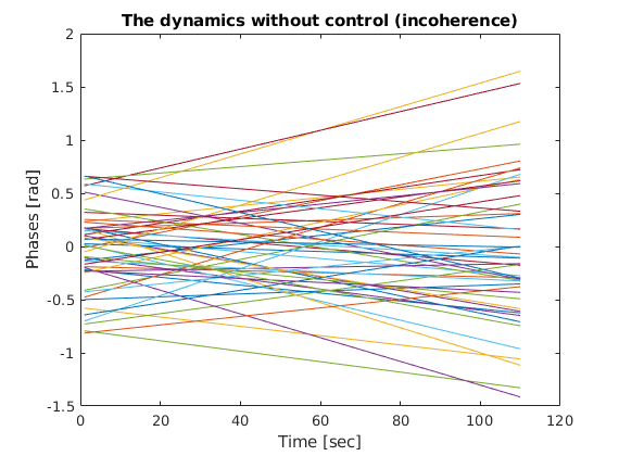
First, we present the dynamics without control,
FreeThetaVector = solve(odeEqn,ControlGuess);
FreeThetaVector = full(FreeThetaVector);
figure
plot(FreeThetaVector')
ylabel('Phases [rad]')
xlabel('Time [sec]')
title('The dynamics without control (incoherence)')
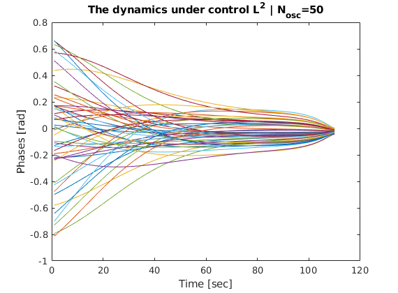
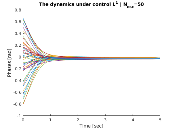
and see the controled dynamics.
figure
plot(OptThetaVector_1')
ylabel('Phases [rad]')
xlabel('Time [sec]')
title("The dynamics under control L^2 | N_{osc}="+m)
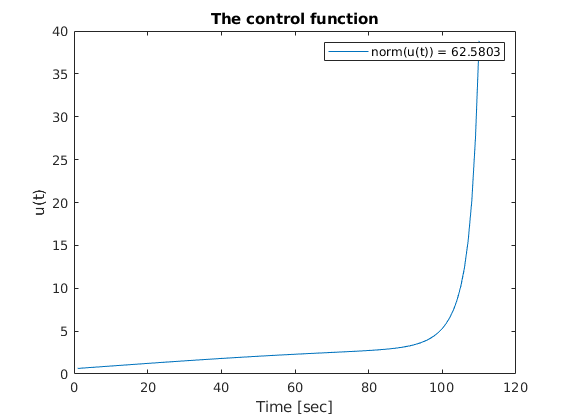
We also can plot the control function along time.
figure
plot(OptControl_1)
legend("norm(u(t)) = "+norm(OptControl_1))
ylabel('u(t)')
xlabel('Time [sec]')
title('The control function')
The problem with different regularization
In this part, we change the regularization into $L^1$-norm and see the difference.
PathCost  = casadi.Function('L'  ,{t,symTh,symU},{ sqrt(symU.^2+1e-3)});
iCP_2 = ocp(odeEqn,PathCost,FinalCost);
tic
[OptControl_2 ,OptThetaVector_2] =  ArmijoGradient(iCP_2,ControlGuess);
toc
Length Step has been change: LenghtStep = 0.00025
iter: 001 | error: 2.363e+01 | LengthStep: 5.00e-04 | J: 1.11735e+02 | Distance2Target: NaN
iter: 002 | error: 2.363e+01 | LengthStep: 1.00e-03 | J: 1.11730e+02 | Distance2Target: NaN
iter: 003 | error: 2.361e+01 | LengthStep: 2.00e-03 | J: 1.11720e+02 | Distance2Target: NaN
iter: 004 | error: 2.359e+01 | LengthStep: 4.00e-03 | J: 1.11699e+02 | Distance2Target: NaN
iter: 005 | error: 2.353e+01 | LengthStep: 8.00e-03 | J: 1.11659e+02 | Distance2Target: NaN
iter: 006 | error: 2.343e+01 | LengthStep: 1.60e-02 | J: 1.11579e+02 | Distance2Target: NaN
iter: 007 | error: 2.322e+01 | LengthStep: 3.20e-02 | J: 1.11420e+02 | Distance2Target: NaN
iter: 008 | error: 2.282e+01 | LengthStep: 6.40e-02 | J: 1.11109e+02 | Distance2Target: NaN
iter: 009 | error: 2.208e+01 | LengthStep: 1.28e-01 | J: 1.10509e+02 | Distance2Target: NaN
iter: 010 | error: 2.081e+01 | LengthStep: 2.56e-01 | J: 1.09388e+02 | Distance2Target: NaN
iter: 011 | error: 1.890e+01 | LengthStep: 5.12e-01 | J: 1.07391e+02 | Distance2Target: NaN
iter: 012 | error: 1.674e+01 | LengthStep: 1.02e+00 | J: 1.04033e+02 | Distance2Target: NaN
iter: 013 | error: 1.607e+01 | LengthStep: 2.05e+00 | J: 9.86861e+01 | Distance2Target: NaN
iter: 014 | error: 4.081e+01 | LengthStep: 4.10e+00 | J: 9.24707e+01 | Distance2Target: NaN
Length Step has been change: LenghtStep = 1.024
Length Step has been change: LenghtStep = 0.256
Length Step has been change: LenghtStep = 0.064
Length Step has been change: LenghtStep = 0.016
Length Step has been change: LenghtStep = 0.004
Length Step has been change: LenghtStep = 0.001
Length Step has been change: LenghtStep = 0.00025
Length Step has been change: LenghtStep = 6.25e-05
Length Step has been change: LenghtStep = 1.5625e-05
Length Step has been change: LenghtStep = 3.9063e-06
Length Step has been change: LenghtStep = 9.7656e-07
Length Step has been change: LenghtStep = 2.4414e-07
Length Step has been change: LenghtStep = 6.1035e-08
Length Step has been change: LenghtStep = 1.5259e-08
Length Step has been change: LenghtStep = 3.8147e-09

    Mininum Length Step have been achive !!

Elapsed time is 2.494788 seconds.
figure

line(tspan,OptThetaVector_2')
ylabel('Phases [rad]')
xlabel('Time [sec]')
title("The dynamics under control L^1 | N_{osc}="+m)
figure
plot(OptControl_1)
line(1:length(OptControl_2),OptControl_2,'Color','red')

Psi_1 = norm(sin(OptThetaVector_1(:,end).' - OptThetaVector_1(:,end)),'fro');
Psi_2 = norm(sin(OptThetaVector_2(:,end).' - OptThetaVector_2(:,end)),'fro');

legend("u(t) with L^2-norm; Terminal cost = "+Psi_1,"u(t) with L^1-norm; Terminal cost = "+Psi_2)
ylabel('The coupling strength (u(t))')
xlabel('Time [sec]')
title('The comparison between two different control cost functionals')
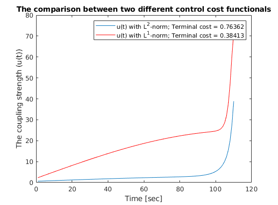
As one can expected from the regularization functions, the control function from $L^2$-norm acting more smoothly from $0$ to the largest value. The function from $L^2$-norm draws much stiff lines.
YFr = FreeThetaVector';
YL1 = OptThetaVector_1';
YL2 = OptThetaVector_2';
%%
animationpendulums({YFr,YL1,YL2},tspan,{'Free','L^2 Control','L^1 Control'})
Finally, we can see the behavior of the two control types against the evolution of free dynamics.