Download Code
In this tutorial we will apply the DyCon toolbox to find a control to the semi-discrete semi-linear heat equation.
where $N^2A$ is the discretization of the Laplacian in 1d in $N$ nodes. We are looking for a control that after time $T$ steers the system near zero.
Setup
In this tutorial we need DyCon Toolbox, to install it we will have to write the following in our MATLAB console:
unzip('https://github.com/DeustoTech/DyCon-Computational-Platform/archive/master.zip')
addpath(genpath(fullfile(cd,'DyCon-toolbox-master')))
Methodology
In order to do so we will frame the problem as a minimization of a functional and we will apply gradient descent to find it. Note that the convexity of the functional is not proven, therefore, we will obtain a local minima for the functional. The functional considered will be:
where by $| \cdot |_{L^2}$ we understand the discrete $L^2$ norm.
Once this control is computed for a certain N, we will think on a dynamical system that models an opinion dynamics with $N$ agents communicating through a chain.
\begin{equation}\label{m1}y_t-\frac{1}{N}Ay=G(y)+Bv\end{equation}
The goal will be to compute also the control $v$ thinking model \eqref{m1} as if it was a semidiscretization of a heat equation with diffusivity $\frac{1}{N^3}$. Furthermore we will also compute the control for model \eqref{m1} with the non-linearity being non-homogeneous on $N$ and a time horizon being $T_N=N^3T$.
clear all
import casadi.*
Definition of the time
ts = SX.sym('t');
%% Discretization of the space
N = 30;
xi = 0; xf = 1;
xline = linspace(xi,xf,N);
Interior Control region between 0.5 and 0.8
w1 = 0.5; w2 = 0.8;
D = 1;
[A,B,count] = GetABmatrix(N,w1,w2,D);
we define symbolically the vectors of the state and the control
Ys = SX.sym('y',[N 1]);
Us = SX.sym('u',[count 1]);
We create the ODE object Our ODE object will have the semi-discretization of the semilinear heat equation. We set also initial conditions, define the non linearity and the interaction of the control to the dynamics.
Initial condition
Diffusion part: the discretization of the 1d Laplacian
Definition of the non-linearity
G = casadi.Function('NLT',{Ys},{10*Ys.*exp(-Ys.^2)});%%
and we define the part of the dynamics corresponding to the nonlinearity
Putting all the things together
F = casadi.Function('F',{ts,Ys,Us},{A*Ys + B*Us + G(Ys)});
%% Creation of the ODE object
%% Time horizon
T = 1;
We create the ODE-object and we change the resolution to $dt=0.01$ in order to see the variation in a small time scale. We will get the values of the solution in steps of size odeEqn.dt, if we do not care about modifying this parameter in the object, we might get the solution in certain time steps that will hide part of the dynamics.
Nt = 100;
tspan = linspace(0,T,Nt);
ipde = semilinearpde1d(Ys,Us,A,B,G,tspan,xline);
ipde.InitialCondition = Y0;
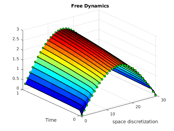
We solve the equation and we plot the free solution applying solve to odeEqn and we plot the free solution.
Yfree = solve(ipde,ZerosControl(ipde));
Yfree = full(Yfree);
figure;
surf(Yfree','EdgeColor','none');
title('Free Dynamics')
xlabel('space discretization')
ylabel('Time')
yticks([1 Nt])
yticklabels([tspan(1) tspan(end)])
We create the object that collects the formulation of an optimal control problem by means of the object that describes the dynamics odeEqn, the functional to minimize Jfun and the time horizon T
L   = Function('L'  ,{ts,Ys,Us},{ Us.'*Us  });
Psi = Function('Psi',{Ys}      ,{ 1e6*(Ys.'*Ys) });

iocp = ocp(ipde,L,Psi);
We apply the steepest descent method to obtain a local minimum (our functional might not be convex).
U0 =ZerosControl(ipde);
[OptControl ,OptState]  = IpoptSolver(iocp,U0);
This is Ipopt version 3.12.3, running with linear solver mumps.
NOTE: Other linear solvers might be more efficient (see Ipopt documentation).

Number of nonzeros in equality constraint Jacobian...:    19236
Number of nonzeros in inequality constraint Jacobian.:        0
Number of nonzeros in Lagrangian Hessian.............:     3900

Total number of variables............................:     3900
                     variables with only lower bounds:        0
                variables with lower and upper bounds:        0
                     variables with only upper bounds:        0
Total number of equality constraints.................:     3000
Total number of inequality constraints...............:        0
        inequality constraints with only lower bounds:        0
   inequality constraints with lower and upper bounds:        0
        inequality constraints with only upper bounds:        0

iter    objective    inf_pr   inf_du lg(mu)  ||d||  lg(rg) alpha_du alpha_pr  ls
   0  3.0000000e+07 9.05e+00 9.67e-01  -1.0 0.00e+00    -  0.00e+00 0.00e+00   0
   1  2.4544321e+05 1.22e-01 7.92e+00  -1.0 3.10e+01  -2.0 1.00e+00 1.00e+00f  1
   2  1.8219937e+06 4.24e-03 1.73e+00  -1.0 1.31e+01  -1.6 1.00e+00 1.00e+00h  1
   3  7.1220860e+04 1.67e-02 2.92e+00  -1.0 9.12e+00  -2.1 1.00e+00 1.00e+00f  1
   4  8.9356500e+03 3.97e-04 8.51e-02  -1.0 2.41e+00  -2.5 1.00e+00 1.00e+00f  1
   5  3.1075917e+03 1.06e-04 3.19e-03  -2.5 2.96e+00  -3.0 1.00e+00 1.00e+00f  1
   6  1.3016546e+03 5.20e-05 1.19e-03  -3.8 3.60e+00  -3.5 1.00e+00 1.00e+00h  1
   7  4.5871538e+02 5.64e-05 4.84e-04  -5.7 4.41e+00  -4.0 1.00e+00 1.00e+00h  1
   8  1.6346578e+02 6.55e-05 1.92e-04  -5.7 5.26e+00  -4.4 1.00e+00 1.00e+00h  1
   9  9.7049320e+01 1.20e-04 3.78e-05  -5.7 3.10e+00  -4.9 1.00e+00 1.00e+00h  1
iter    objective    inf_pr   inf_du lg(mu)  ||d||  lg(rg) alpha_du alpha_pr  ls
  10  4.0069187e+01 9.26e-03 1.98e-05  -5.7 1.48e+01    -  1.00e+00 5.00e-01h  2
  11  1.6748754e+01 4.28e-04 2.92e-06  -5.7 4.34e+00    -  1.00e+00 1.00e+00h  1
  12  1.6371256e+01 4.58e-06 9.87e-09  -5.7 1.88e-01    -  1.00e+00 1.00e+00h  1
  13  1.6367177e+01 1.03e-11 1.11e-13  -8.6 7.84e-04    -  1.00e+00 1.00e+00h  1

Number of Iterations....: 13

                                   (scaled)                 (unscaled)
Objective...............:   8.1835886066017175e-04    1.6367177213203433e+01
Dual infeasibility......:   1.1096830919432588e-13    2.2193661838865175e-09
Constraint violation....:   1.0345974077452524e-11    1.0345974077452524e-11
Complementarity.........:   0.0000000000000000e+00    0.0000000000000000e+00
Overall NLP error.......:   1.0345974077452524e-11    2.2193661838865175e-09


Number of objective function evaluations             = 19
Number of objective gradient evaluations             = 14
Number of equality constraint evaluations            = 19
Number of inequality constraint evaluations          = 0
Number of equality constraint Jacobian evaluations   = 14
Number of inequality constraint Jacobian evaluations = 0
Number of Lagrangian Hessian evaluations             = 13
Total CPU secs in IPOPT (w/o function evaluations)   =      0.436
Total CPU secs in NLP function evaluations           =      0.057

EXIT: Optimal Solution Found.
               t_proc [s]   t_wall [s]    n_eval
       nlp_f     0.000826     0.000828        19
       nlp_g      0.00916      0.00917        19
  nlp_grad_f      0.00139      0.00139        15
  nlp_hess_l       0.0175       0.0174        13
   nlp_jac_g       0.0333       0.0333        15
      solver        0.507        0.501         1
Elapsed time is 0.636870 seconds.
plotSHE(OptState,OptControl,Yfree,YT,xline,tspan,Nt)
Collective behavior dynamics
Now we apply the same procedure for the collective behavior dynamics. We will employ a function that does the algorithm explained before for the semilinear heat equation having the chance to set a diffusivity constant.
For the simulation of the model in collective behavior we will employ a diffusivity $D=\frac{1}{N^3}$.
D = 1/(N^3);
[A,B,count] = GetABmatrix(N,w1,w2,D);
%%
G = casadi.Function('NLT',{Ys},{10*Ys.*exp(-Ys.^2)});%%
%%
T = 1;  Nt = 100;
tspan = linspace(0,T,Nt);
%%
ipde = semilinearpde1d(Ys,Us,A,B,G,tspan,xline);
ipde.InitialCondition = Y0;
%%
iocp = ocp(ipde,L,Psi);
U0 =ZerosControl(ipde);
%%[OptControl ,OptState]  = ArmijoGradient(iocp,U0,'MaxIter',200);
[OptControl ,OptState]  = IpoptSolver(iocp,U0);
This is Ipopt version 3.12.3, running with linear solver mumps.
NOTE: Other linear solvers might be more efficient (see Ipopt documentation).

Number of nonzeros in equality constraint Jacobian...:    19236
Number of nonzeros in inequality constraint Jacobian.:        0
Number of nonzeros in Lagrangian Hessian.............:     3900

Total number of variables............................:     3900
                     variables with only lower bounds:        0
                variables with lower and upper bounds:        0
                     variables with only upper bounds:        0
Total number of equality constraints.................:     3000
Total number of inequality constraints...............:        0
        inequality constraints with only lower bounds:        0
   inequality constraints with lower and upper bounds:        0
        inequality constraints with only upper bounds:        0

iter    objective    inf_pr   inf_du lg(mu)  ||d||  lg(rg) alpha_du alpha_pr  ls
   0  3.0000000e+07 1.00e+00 9.72e-01  -1.0 0.00e+00    -  0.00e+00 0.00e+00   0
   1  1.1211823e+08 6.93e-02 1.07e+01  -1.7 1.75e+00   0.0 1.00e+00 1.00e+00h  1
   2  1.0201471e+08 2.53e-02 2.23e+00  -1.7 3.50e+00  -0.5 1.00e+00 1.00e+00f  1
   3  8.8642262e+07 4.18e-02 5.31e-01  -1.7 2.13e+02    -  1.00e+00 1.00e+00f  1
   4  8.2505158e+07 1.39e+00 3.13e+00  -1.7 2.72e+03    -  1.00e+00 1.00e+00F  1
   5  7.9212105e+07 9.68e+00 5.20e+00  -1.7 1.38e+03    -  1.00e+00 1.00e+00f  1
   6  7.8291279e+07 6.94e-02 2.84e+00  -1.7 2.05e+03    -  1.00e+00 1.00e+00f  1
   7  7.8090072e+07 1.57e+00 4.98e-01  -1.7 7.87e+02    -  1.00e+00 1.00e+00f  1
   8  7.8026943e+07 1.54e-01 8.25e-02  -1.7 3.33e+02    -  1.00e+00 1.00e+00f  1
   9  7.8491521e+07 4.41e-02 7.64e+00  -2.5 2.10e+00  -1.0 1.00e+00 1.00e+00h  1
iter    objective    inf_pr   inf_du lg(mu)  ||d||  lg(rg) alpha_du alpha_pr  ls
...
...
  54  7.8022238e+07 4.03e-07 8.33e-10  -5.7 2.15e-02    -  1.00e+00 1.00e+00h  1
  55  7.8022238e+07 9.83e-12 1.82e-12  -8.6 1.02e-04    -  1.00e+00 1.00e+00h  1

Number of Iterations....: 55

                                   (scaled)                 (unscaled)
Objective...............:   3.9011119130960064e+03    7.8022238261920124e+07
Dual infeasibility......:   1.8189894035458565e-12    3.6379788070917130e-08
Constraint violation....:   9.8296371042749797e-12    9.8296371042749797e-12
Complementarity.........:   0.0000000000000000e+00    0.0000000000000000e+00
Overall NLP error.......:   9.8296371042749797e-12    3.6379788070917130e-08


Number of objective function evaluations             = 111
Number of objective gradient evaluations             = 56
Number of equality constraint evaluations            = 111
Number of inequality constraint evaluations          = 0
Number of equality constraint Jacobian evaluations   = 56
Number of inequality constraint Jacobian evaluations = 0
Number of Lagrangian Hessian evaluations             = 55
Total CPU secs in IPOPT (w/o function evaluations)   =      1.374
Total CPU secs in NLP function evaluations           =      0.308

EXIT: Optimal Solution Found.
               t_proc [s]   t_wall [s]    n_eval
       nlp_f      0.00624      0.00627       111
       nlp_g       0.0634       0.0633       111
  nlp_grad_f      0.00762      0.00768        57
  nlp_hess_l       0.0868       0.0846        55
   nlp_jac_g        0.149        0.149        57
      solver         1.74         1.73         1
Elapsed time is 1.874814 seconds.
plotSHE(OptState,OptControl,Yfree,YT,xline,tspan,Nt)
Now we will change also the time horizon and we will incorporate a non-homogeneous non-linearity, we will just divide the non-linearity $G$ by $N^3$
D = 1/(N^2);
[A,B,count] = GetABmatrix(N,w1,w2,D);
%%
G = casadi.Function('NLT',{Ys},{10*Ys.*exp(-Ys.^2)/N^2} );%%
%%
T = N^2;  Nt = 100;
tspan = linspace(0,T,Nt);
%%
ipde = semilinearpde1d(Ys,Us,A,B,G,tspan,xline);
ipde.InitialCondition = Y0;
%%
iocp = ocp(ipde,L,Psi);
U0 =ZerosControl(ipde);
[OptControl ,OptState]  = IpoptSolver(iocp,U0);
This is Ipopt version 3.12.3, running with linear solver mumps.
NOTE: Other linear solvers might be more efficient (see Ipopt documentation).

Number of nonzeros in equality constraint Jacobian...:    19236
Number of nonzeros in inequality constraint Jacobian.:        0
Number of nonzeros in Lagrangian Hessian.............:     3900

Total number of variables............................:     3900
                     variables with only lower bounds:        0
                variables with lower and upper bounds:        0
                     variables with only upper bounds:        0
Total number of equality constraints.................:     3000
Total number of inequality constraints...............:        0
        inequality constraints with only lower bounds:        0
   inequality constraints with lower and upper bounds:        0
        inequality constraints with only upper bounds:        0

iter    objective    inf_pr   inf_du lg(mu)  ||d||  lg(rg) alpha_du alpha_pr  ls
   0  3.0000000e+07 9.05e+00 1.17e+02  -1.0 0.00e+00    -  0.00e+00 0.00e+00   0
   1  2.8754020e+04 1.48e-01 4.01e+00  -1.0 2.73e+00   0.0 1.00e+00 1.00e+00f  1
   2  3.0839145e+03 1.91e-02 3.08e-01  -1.0 9.19e-01  -0.5 1.00e+00 1.00e+00h  1
   3  9.2703794e+02 1.17e-03 2.31e-02  -1.7 2.08e-01  -1.0 1.00e+00 1.00e+00h  1
   4  4.2707593e+02 2.49e-03 9.65e-03  -3.8 2.61e-01  -1.4 1.00e+00 1.00e+00h  1
   5  2.2851845e+02 1.36e-03 2.60e-03  -3.8 2.10e-01  -1.9 1.00e+00 1.00e+00h  1
   6  1.5158663e+02 1.25e-03 9.80e-04  -3.8 2.38e-01  -2.4 1.00e+00 1.00e+00h  1
   7  1.0229631e+02 2.37e-03 4.26e-04  -5.7 3.11e-01  -2.9 1.00e+00 1.00e+00h  1
   8  8.6220145e+01 1.84e-01 3.73e-04  -5.7 2.84e+01    -  1.00e+00 1.25e-01h  4
   9  1.6663658e+00 6.98e-02 4.71e-05  -5.7 2.20e+00    -  1.00e+00 1.00e+00h  1
iter    objective    inf_pr   inf_du lg(mu)  ||d||  lg(rg) alpha_du alpha_pr  ls
  10  1.1303218e-01 1.61e-02 9.28e-07  -5.7 4.53e-01    -  1.00e+00 1.00e+00h  1
  11  3.7959122e-02 7.79e-03 2.54e-08  -5.7 2.84e-01    -  1.00e+00 1.00e+00h  1
  12  2.1316195e-02 1.77e-03 4.98e-09  -5.7 1.39e-01    -  1.00e+00 1.00e+00h  1
  13  1.8447375e-02 6.30e-06 5.26e-11  -5.7 8.15e-03    -  1.00e+00 1.00e+00h  1
  14  1.8440851e-02 2.26e-09 9.54e-15  -8.6 1.61e-04    -  1.00e+00 1.00e+00h  1

Number of Iterations....: 14

                                   (scaled)                 (unscaled)
Objective...............:   9.2204254694796125e-07    1.8440850938959225e-02
Dual infeasibility......:   9.5381182640930876e-15    1.9076236528186175e-10
Constraint violation....:   2.2559639156760625e-09    2.2559639156760625e-09
Complementarity.........:   0.0000000000000000e+00    0.0000000000000000e+00
Overall NLP error.......:   2.2559639156760625e-09    2.2559639156760625e-09


Number of objective function evaluations             = 19
Number of objective gradient evaluations             = 15
Number of equality constraint evaluations            = 19
Number of inequality constraint evaluations          = 0
Number of equality constraint Jacobian evaluations   = 15
Number of inequality constraint Jacobian evaluations = 0
Number of Lagrangian Hessian evaluations             = 14
Total CPU secs in IPOPT (w/o function evaluations)   =      0.415
Total CPU secs in NLP function evaluations           =      0.065

EXIT: Optimal Solution Found.
               t_proc [s]   t_wall [s]    n_eval
       nlp_f     0.000898     0.000903        19
       nlp_g      0.00904      0.00905        19
  nlp_grad_f       0.0017      0.00169        16
  nlp_hess_l       0.0214       0.0214        14
   nlp_jac_g       0.0354        0.035        16
      solver        0.489        0.487         1
Elapsed time is 0.616536 seconds.
plotSHE(OptState,OptControl,Yfree,YT,xline,tspan,Nt)