Download Code
This tutorial aims to show how to build equations of motion, control system model and optimally stabilizing controllers for the inverted pendulum. This tutorial is a standard material in control engineering education. We first derive the equations of motion via Lagrange’s method using Symbolic Math Toolbox. Then, a linear control model is derived. The optimal controller is designed using linear quadratic regulator theory. Simulations are carried out for the inverted pendulum nonlinear model. In Appendix, finite horizon linear optimal control is shown by solving a differential Riccati equation.
A schematic of an inverted pendulum is shown below.
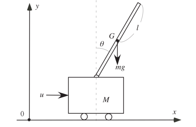
A pendulum is attached with a cart that moves horizontally due to the force $u$ without friction. The pendulum freely rotates around the pivot on the cart. It is assumed that the cart and pendulum move in the vertical plane. The masses of the pendulum and cart are $m$ and $M$, respectively, and the length of the pendulum is $2l$. The position of the cart is denoted by $x$ and the angle of the pendulum from the vertical axis is $\theta$.
syms t;
syms x dx theta dtheta;
syms M m l g;
syms Lgr Lgr_x Lgr_dx Lgr_theta Lgr_dtheta;
Derivation of equations of motion
The Lagrangian $L$ consists of the kinetic energy and potential energy, which is given by
Lgr = 1/2 * M*dx^2 + 2/3 * m*l^2*dtheta^2 + m*l*dx*dtheta*cos(theta)...
        + 1/2 *m*dx^2 - m*g*l*cos(theta);
Compute derivatives of Lagrangian
Lgr_x = diff(Lgr,x);
Lgr_dx = diff(Lgr,dx);
Lgr_theta = diff(Lgr,theta);
Lgr_dtheta = diff(Lgr,dtheta);

syms x_f(t) dx_f(t) theta_f(t) dtheta_f(t) Lgr_x_f Lgr_dx_f Lgr_theta_f Lgr_dtheta_f; %% _f means functionalized
dx_f(t)=diff(x_f,t);
dtheta_f=diff(theta_f,t);

Lgr_dx_f = subs(Lgr_dx,[x dx theta dtheta],[x_f dx_f theta_f dtheta_f])
Lgr_theta_f = subs(Lgr_theta,[x dx theta dtheta],[x_f dx_f theta_f dtheta_f])
Lgr_dtheta_f = subs(Lgr_dtheta,[x dx theta dtheta],[x_f dx_f theta_f dtheta_f])
Lgr_dx_f =

M*diff(x_f(t), t) + m*diff(x_f(t), t) + l*m*cos(theta_f(t))*diff(theta_f(t), t)


Lgr_theta_f =

g*l*m*sin(theta_f(t)) - l*m*sin(theta_f(t))*diff(theta_f(t), t)*diff(x_f(t), t)


Lgr_dtheta_f =

(4*m*diff(theta_f(t), t)*l^2)/3 + m*cos(theta_f(t))*diff(x_f(t), t)*l
Coumpute Lagrange’s equations of motion with external force $u$
syms Leq Eqn;
Leq = diff([Lgr_dx_f; Lgr_dtheta_f],t) - [Lgr_x; Lgr_theta_f];
syms Ddx Ddtheta u;
Leq = subs(Leq,[diff(x_f(t), t, t) , diff(theta_f(t), t, t) ],[Ddx, Ddtheta])-[u; 0];
Eqn = solve(Leq==0,[Ddx,Ddtheta]);
Construct state space equations of the first order equation
syms x1 x2 x3 x4 X;
X = [x1;x2;x3;x4];
subs(Eqn.Ddx, [x_f, diff(x_f(t),t), theta_f, diff(theta_f(t),t)], [x1, x2, x3, x4]);
subs(Eqn.Ddtheta, [x_f, diff(x_f(t),t), theta_f, diff(theta_f(t),t)], [x1, x2, x3, x4]);

syms Nsys
Nsys = [x2;...
        subs(Eqn.Ddx, [x_f, diff(x_f(t),t), theta_f, diff(theta_f(t),t)], [x1, x2, x3, x4]);...
        x4;...
        subs(Eqn.Ddtheta, [x_f, diff(x_f(t),t), theta_f, diff(theta_f(t),t)], [x1, x2, x3, x4])];

syms F;
F = subs(Nsys,u,0);
Construct linear model $\dot{x} = Ax+Bu$
syms Amat Bmat
Amat = subs(jacobian(F,X),[x1,x2,x3,x4],[0,0,0,0])
Bmat = diff(subs(Nsys,[x1,x2,x3,x4],[0,0,0,0]),u)
Amat =

[ 0, 1,                             0, 0]
[ 0, 0,            -(3*g*m)/(4*M + m), 0]
[ 0, 0,                             0, 1]
[ 0, 0, (3*(M*g + g*m))/(l*(4*M + m)), 0]


Bmat =

                0
      4/(4*M + m)
                0
 -3/(l*(4*M + m))
We will use the following physical parameters m = 0.3 [kg]; M = 0.8 [kg]; l = 0.25 [m]; g = 9.8 [m/s^2];
A = double(subs(Amat,[m M l g],[0.3 0.8 0.25 9.8]));
B = double(subs(Bmat,[m M l g],[0.3 0.8 0.25 9.8]));
LQR controller design
We design a linear feedback controller that minimizes the cost function
R = 1; Q = diag([1,1,1,1]);
[ricsol,cleig,K,report] = care(A,B,Q);

f_ctr = @(x) -K*x;
i_linear = @(t,x) A*x + B*f_ctr(x); %% closed loop systems

tspan = [0,10];
ini =[0,0,0.91,0]; %%1.1894299
[time, state] = ode45(i_linear,tspan, ini);
input_linear = f_ctr(state');
Simulations with linear and nonlinear models
Nsys_f = matlabFunction(Nsys); %% function of M,g,l,m,u,x2,x3,x4
i_nonlinear = @(t,x) Nsys_f(0.8,9.8,0.25,0.3,f_ctr(x),x(2),x(3),x(4));

[timen, staten] = ode45(i_nonlinear,tspan, ini);
input_nonlinear = f_ctr(staten');
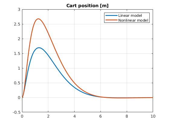
clf
plot(time, state(:,1),'LineWidth',2)
hold on
plot(timen, staten(:,1),'LineWidth',2)
grid on
legend('Linear model', 'Nonlinear model')
title('Cart position [m]')
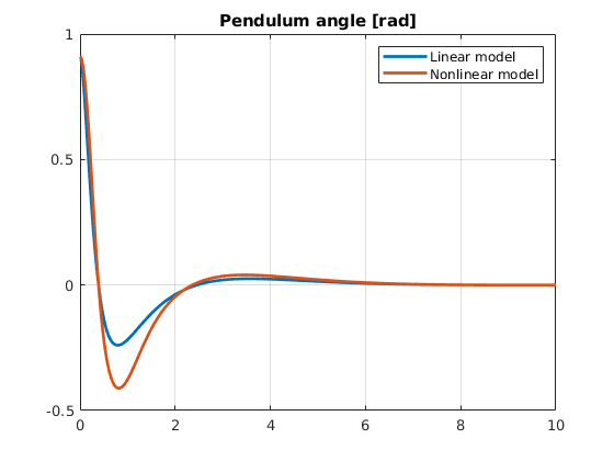
clf
plot(time, state(:,3),'LineWidth',2)
hold on
plot(timen, staten(:,3),'LineWidth',2)
grid on
legend('Linear model', 'Nonlinear model')
title('Pendulum angle [rad]')
clf
plot(time, input_linear,'LineWidth',2)
hold on;grid on
plot(timen, input_nonlinear,'LineWidth',2)
legend('Linear model','Nonlinear model')
title('Input response')
Appendix (finite interval optimal control with DRE )
rho = 0;
S = rho * eye(size(A,1));
Solve -dX/dt = XA + A’X - XBR^{-1}B’X +Q, X(T) = S (DRE)
tspan_ric = [10,0]; %% change horizon!
iniric = S(:);
i_ric = @(t,x) -f_dric(x, A, B * B.', Q);
opts = odeset('RelTol',1e-10,'AbsTol',1e-10);
[time_ric, X] = ode45(i_ric, tspan_ric, iniric, opts);
reshape(X(end,:),4,4)-ricsol %% Convergence check with sol of ARE
ans =

   1.0e-04 *

   -0.0103   -0.0124   -0.0358   -0.0065
   -0.0124   -0.0185   -0.0549   -0.0099
   -0.0358   -0.0549   -0.1639   -0.0295
   -0.0065   -0.0099   -0.0295   -0.0053
Construct feedback controller using interpolation of DRE sol
gain = zeros(length(X),size(A,1));
for i = 1:length(X)
    gain(i,:) = B' * reshape(X(i,:),size(A));
end
gain_t = @(t) interp1(time_ric,gain,t);
u_dr = @(t,x) -gain_t(t)*x;

tspan = sort(tspan_ric, 'ascend');
i_nonlinear_dre = @(t,x) Nsys_f(0.8,9.8,0.25,0.3,u_dr(t,x),x(2),x(3),x(4));
[timedn, statedn] = ode45(i_nonlinear_dre,tspan, ini);%%
input_dric=[];
for i = 1:length(timedn)
    input_dric(i) = u_dr(timedn(i),statedn(i,:)');
end
clf
plot(timedn, statedn(:,3),'LineWidth',2)
grid on
hold on
plot(timen, staten(:,3),'ro')
legend('control with DRE [10,0]', 'control with ARE')
title('Pendulum responses with nonlinear model')
hold off
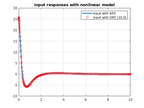
plot(timedn,input_dric,'LineWidth',2)
hold on
plot(timen,input_nonlinear,'ro')
grid on
legend('input with ARE','input with DRE [10,0]')
title('input responses with nonlinear model')