Download Code
We design a LQR controller for stabilyzing the fractional reaction diffusion equation
where $\delta>0$ is a given constant, $\omega = (a,b)\subset(-L,L)$ and $(-d_x^2)^s$, $s\in(0,1)$ denotes the one-dimensional fractional Laplacian defined as
with $c(s)$ an explicit normalization constant.
When considering this equation without the action of the the control $u$, we know that, depending on the value of $\delta$, the corresponding dynamics may become unstable. This is due to the fact that the eignenvalues of the associated elliptic problem are given by $\mu_k=c-\lambda_k$ ($\lambda_k$ being the eigenvalues of the fractional Laplacian on $(-L,L)$ with zero Dirichlet boundary conditions), and they are positive if $c>\lambda_1$ (since, in addition, we know that $\lambda_1<\lambda_k$ for all $K$). We are then intersted in designing a LQR control which is able to stabilyze this solution and prevent its blow-up.
The computation of the LQR control is carried out by means of the following procedure:
STEP 1. Discretization of the equation
We start by discretizing our original system on a uniform mesh $x_i$, $i=1,\ldots,N$, thus obtaining a N-dimensional system of the type
where:
-
with some abuse of notation, we denoted $y\in\mathbb{R}^N$ as the $N$-dimensional vector whose entries $y_i=y(x_i)$, $i=1,\ldots,N$ are the evaluation of the function $y$ on the points of the mesh;
-
the matrix $A$ is a discretization of the operator $-(-d_x^2)^s + I$, $I$ denoting the identity;
-
the matrix $B$ defines the action of the control.
The computation of the matrix requires the discretization of the fractional Laplacian $(-d_x^2)^s$. This is done by employing the function “fl_rigidity”, which implements a finite elements method on a uniform mesh discretizing the space interval $(-L,L)$ (complete details on this method may be found in [1]).
The function “fl_rigidity” works by requiring 3 input parameters:
-
s: the order of the fractional Laplacian, which can be any real value in the interval $(0,1)$;
-
L: any real value, defining the extrema of the space interval $(-L,L)$;
-
N: the number of discretization points in the mesh employed.
The outputs are:
The matrix B, instead, is constructed by employing the function “construction_matrix_B”, which takes in input
-
the vector $x$ containing the mesh;
-
the number of discretization points $N$;
-
the characteristic function of the sub-interval $\omega$.
STEP 2. Definition of the cost functional and computation of the control
Once we have the semi-discretization of our original problem, the control we are looking for is computed by minimizing the following cost functional
where $Q\geq 0$ and $R>0$ are given matrices. Moreover, we know that this control is given in a feedback form by $u^*=-R^{-1}B^TPy$, where $P$ is the solution of the algebraic Riccati equation
Implementation
We start by defining the parameter $s\in(0,1)$ (order of the fractional Laplacian), the size of the interval $(-L,L)$, the constant $\delta> \lambda_1$ and the number $N$ of discretization points in our mesh.
s = 0.8;
L = 1;
d = (0.5*pi)^(2*s)+0.1;
N = 100;
and we compute the corresponding approximation of the fractional Laplacian
[x,FL] = fl_rigidity(s,L,N);
We then use it for building the matrix $A$ describing the dynamics
Secondly, we use the function “construction_matrix_B” for computing the control operator $B$ on the interval $\omega=(-0.3,0.5)$
matrix_B =  @(x) interval(x,-0.3,0.5);
B = construction_matrix_B(x,N,matrix_B);
Out of the matrices $A$ and $B$, we solve the algebraic Riccati equation by employing the specific function from the control systems toolbox of Matlab. For simplicity, we choose both $R$ and $Q$ as the identity, but other choices are possible in order to improve the efficiency of the method.
R = eye(N);
Q = eye(N);
[P,cleig,K,report] = care(A,B,eye(N));
The output matrix $K=-R^{-1}B^TP$ is used for defining the action of the control and include it in our system
f_ctr = @(x) -K*x;
eq_ctr = @(t,x) A*x + B*f_ctr(x);
Finally, we choose an initial datum
and we solve our equation with and without control employing the “ode45” function of Matlab. For the equation without control we choose a relatively short time horizon, since we know that the unstable dynamics will rapidly diverge. For the equation with control, instead, we choose a longer time horizon in order to have enough time for stabilyzing the system.
T1 = 4;
T2 = 25;
Nt = 40;
tspan1 = linspace(0,T1,Nt);
tspan2 = linspace(0,T2,Nt);
eq_free = @(t,x) A*x;
[time1, sol_free] = ode45(eq_free,tspan1,y0);
[time2, sol_ctr] = ode45(eq_ctr,tspan2,y0);
We then plot our results and compare them. Firstly, the free dynamics.
surf(x,time1,sol_free)
colormap jet
msol_free = floor(min(min(sol_free)));
Msol_free = round(max(max(sol_free)));
xticks([-L L])
yticks([0 T1])
zticks([msol_free Msol_free])
view(135,25)
title('Free unstable dynamics')
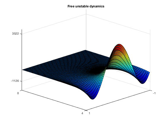
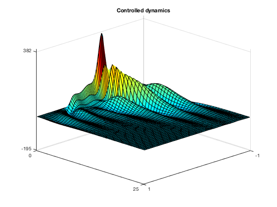
We clearly see the growth of the solution, already in the short time horizon [0,4]. When introducing the LQR control, instead, the problem is corrected and the equation is stabilyzed in time $T_2$
surf(x,time2,sol_ctr)
colormap jet
msol_ctr = floor(min(min(sol_ctr)));
Msol_ctr = round(max(max(sol_ctr)));
xticks([-L,L])
yticks([0 T2])
zticks([msol_ctr Msol_ctr])
view(135,25)
title('Controlled dynamics')
References
[1] U. Biccari and V. Hernandez-Santamaria, “Controllability of a one-dimensional fractional heat equation: theoretical and nuerical aspects”, IMA J. Math. Control I. (2018).