Q-learning for finite-dimensional problems

Reinforcement Learning

Reinforcement Learning (RL) is, together with Supervised Learning and Unsupervised Learning, one of the three fundamental learning paradigms in Machine Learning. The goal in RL is to enhance the manipulation of a controlled system by using data from past experiments. It differs from supervised learning and unsupervised learning because the algorithms are not trained with a fixed sampled dataset. Rather, they learn through trial and error.

In a generic RL problem, an agent, or decision maker, interacts with an unknown environment which is influenced and evolves according to the controls, or actions, that are chosen by the agent. The control chosen in each situation is then evaluated by means of a reward signal. Based on the experience acquired in previous trials, the algorithm has to learn what actions are better in each situation, in the sense that the accumulated long-time reward is maximized.

An optimal control problem

From a mathematical viewpoint, we can see RL as an optimal control problem. The environment is described through a dynamical system of the form

$\tag{1} \left\{ \begin{array}{ll} x_{t+1} = f(x_t,u_t) & t= 0,1,2,\ldots \\ x_0 = x \end{array} \right.$

At each time-step, $x_t$ represents the state of the environment, which evolves according to the function $f: \mathbb{R}^n\times \mathcal{U} \to \mathbb{R}^n$. This function might be unknown by the agent, and depends on the current state $x_t$ and the control $u_t$ chosen by the agent. This choice is then evaluated by a reward $r_t = r(x_t,u_t)$.

The reward function $r: \mathbb{R}^n\times \mathcal{U}\to \mathbb{R}$ has to be designed in such a way that the desired behavior of the system is stimulated by providing greater rewards. It is important to note that the choice of $u_t$ not only affects the reward $r_t$. It also affects the future rewards as they will depend on future states of the system. The goal in RL is not to maximize the reward $r_t$ at each time-step, but rather to maximize the reward accumulated during a certain interval of time.

The optimal control problem that we are considering consists in maximizing, over the control strategy, the rewards accumulated during a process of infinite length

$\tag{2} \max_{\{u_t\}_t} \sum_{t=0}^\infty \gamma^t r(x_t,u_t) \qquad \text{subject to (1)}.$

The parameter $\gamma \in (0,1)$ is called a discount factor, and ensures that the sum of rewards over the time-steps is finite. This is the so-called discounted infinite-horizon problem. In many applications, the introduction of the discount factor is also motivated by the fact that the rewards obtained in the near future are considered to be more important than those obtained with a bigger delay.

It is to be pointed out that this general setting is not exhaustive, and other classes of optimal control problems can be considered in the application of RL techniques. For example, it is typical to consider stochastic dynamics, which is very suitable when the environment is considered to be unknown, or is subject to changes that we cannot control. The reward functional (2) can also have a different form (finite-time horizon, terminal reward, no discount factor,…). Although the discrete-time setting is the most common in RL, continuous-time problems can also considered.

The value function

The probably most important element in Reinforcement Learning is the optimal value function, defined as

$V^\ast (x) := \max_{\{u_t\}_t} \left\{ \sum_{t=0}^\infty \gamma^t r(x_t,u_t); \quad \text{s.t. (1) with $x_0 = x$} \right\}$

It represents the best total reward that one can expect if the initial state is $x$. The value function satisfies the following Dynamic Programming Principle, also known as Bellman equation.

$V^\ast (x) = \max_{u\in \mathcal{U}} \left\{ r(x,u) + \gamma V^\ast (f(x,u)) \right\}$

It allows the design of an optimal control in a feedback form.

$\tag{3} u^\ast (x) = \text{argmax}_{u\in \mathcal{U}} \left\{ r(x,u) + \gamma V^\ast (f(x,u)) \right\}$

The $Q$-function

In view of (3), we can construct a nearly optimal feedback control by approximating the value function $V^\ast$. But even if we were able to exactly compute the value function, the feedback law given in (3) makes use of the dynamics $f$. This means that the choice of the optimal control at a given state relies on the possibility of making predictions of what will be the next state, and as we mentioned, it is not in general the case in RL.

Therefore, rather than approximating the value function, we may concentrate our efforts on approximating the $Q$-function, defined as

$Q(x,u) := r(x,u) + \gamma V^\ast (f(x,u))$

It represents the best total reward that we can expect if the initial state is $x$ and the first control taken is $u$.

Observe that the optimal value function $V^\ast(x)$ determines how good is to be at a certain state $x$, whereas the function $Q(x,u)$ determines the quality of choosing $u$ given that the current state is $x$.

The $Q$-function allows the design of an optimal feedback control without using the dynamics $f$.

$u^\ast (x) = \text{argmax}_{u\in \mathcal{U}} Q(x,u)$

Using the identity $V^\ast (x) = \max_{u\in \mathcal{U}} Q(x,u)$, we can deduce the Bellman equation for the $Q$-function.

$\tag{4} Q(x,u) = r(x,u) + \gamma \max_{u\in \mathcal{U}} Q(x,u)$

$Q$-learning

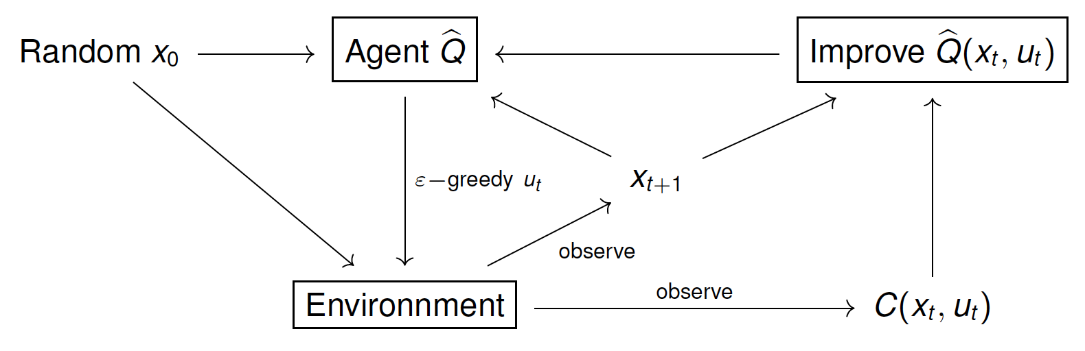
$Q$-learning is a RL algorithm, introduced by Watkins in 1989, that seeks to approximate the $Q$-function by exploring the state-control space $\mathbb{R}^n\times \mathcal{U}$. The exploration is made by running experiments of finite time-steps considering a randomized initial state. At each step, the approximation of the $Q$-function is improved by using the Dynamic Programming equation (4). During the learning process, an $\varepsilon$-greedy policy with respect to the current approximation of $Q$ is used. This policy ensures the exploration of the whole state-control space at the same time that it exploits the information obtained in previous experiments to enhance the approximation of $Q$ in regions that seem to be better in terms of total reward.

These are the main steps in the $Q$-learning algorithm.

Initialize an arbitrary $Q$-function, $\widehat{Q}_0(x,u)$.
Run a number $N$ of experiments (episodes) of $T$ steps each one.
In total there will be $N\, T$ number of steps.
$\varepsilon$-greedy policy:

$u_t = \max_{u\in\mathcal{U}} \widehat{Q}_k(x_t,\, u)\quad \text{with probability $1-\varepsilon$}$

and $u_k$ is chosen randomly with probability $\varepsilon$ (exploration vs exploitation).

Improvement of $\widehat{Q}(x_t, u_t)$: after each time-step, we use the observed $(x_{t+1}, r_t)$ to improve the approximation of $Q(x_t,u_t)$ in the following way

$\widehat{Q}_{k+1} (x_t,u_t) = (1-\alpha) \widehat{Q}_k(x_t,u_t) + \alpha \big( r_t + \gamma \max_{u\in\mathcal{U}} \widehat{Q}_k(x_{t+1}, u) \big)$

here, $\alpha>0$ is called the learning rate.


Figure 1.

Example

We illustrate the $Q$-learning algorithm through a simple example. In a given two-dimensional discrete domain, we consider the problem of finding the shortest path between any position of the domain and a prescribed target area.

Let us first define the environment. We consider a discretized rectangular domain:

$\Omega := \{ 1,2,3, \ldots, 40 \}^2$

We want to find the shortest path between any starting position in the domain and the top center of the domain, white area in the video below. The position can be moved, at each time-step, one unit up, down, right or left, i.e. the underlying dynamics are given by

$\left\{ \begin{array}{l} x_{t+1} = x_t + u_t \quad t = 0,1,2, \ldots ,\tau \\ x_0 = x \end{array} \right.$

where $\tau$ is the first time the state reaches the limits of the domain. The experiment is considered a success if the terminal position is in the target area, and a defeat otherwise. The possible controls are

$\mathcal{U}:= \{ (0,1), -(0,1), (1,0), -(1,0) \}$

We denote by $\partial \Omega$ the limits of the domain (blue squares in the video), i.e.

$\partial \Omega := \{ (i,j) \in \Omega\, ; \text{with} \ \{ i, j\} \cap \{1,40\} \neq \emptyset \}$

We denote by $\mathcal{T}$ the target area (white squares)

$\mathcal{T} := \{ (1,j) \in \Omega\, ; j\in [18,22] \}$

Now we need to define a reward that makes the agent move the position from the initial one $x$ to the target area in the minimum number of steps, without reaching the limits of the domain.

$r(x_t,u_t):= \left\{ \begin{array}{ll} -1 & \text{if} \ x_t \in \Omega \\ 100 & \text{if} \ x_t \in \mathcal{T} \\ -100 & \text{if} \ x_t \in \partial\Omega \setminus \mathcal{T} \end{array} \right.$

Giving a negative reward when $x_t\in \Omega$ stimulates the agent to take the minimum possible number of steps until the target area.

Since the state-space $\Omega$ and the set of possible actions $\mathcal{U}$ are both finite. The $Q$-function can be represented by a table with $40\times 40$ rows and $4$ columns. The entries in this table can be learned from experiments using the $Q$-learning algorithm described above. Once we have a good approximation of $Q$, for a given position $x$, we can determine the best possible action by looking at the corresponding row in the table and taking the action corresponding to the minimum value in that row.

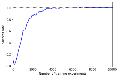
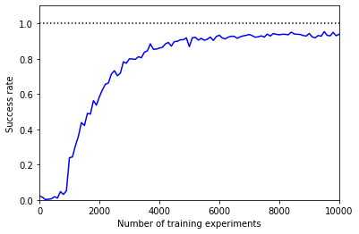
In the following video we see the obtained behavior after applying the $Q$-learning algorithm with 10000 experiments, with a discount factor $\gamma =0.9$, learning rate $\alpha =0.9$ and an $\varepsilon-$greedy policy with $\varepsilon = 0.9$. The plot represents the evolution of the success rate with the number of experiments during the training.


Figure 2a.	Figure 2b.

We can change the environment by adding a potential that moves the position to the right when it is in a certain region (dark green area)

$P: = \{ (i,j)\in \Omega \, ; j\in [5,15] \}$

In the new environment, the agent do not know how to get to the target area.

In the following video, the agent uses the $Q$-function obtained in the original environment. However, the new dynamics are given by

$x_{t+1} = \left\{ \begin{array}{ll} x_t + u_t & \text{if} \ x_t\in \Omega\setminus P \\ x_t +3+ u_t & \text{if} \ x_t\in P \end{array} \right.$

Figure 3.

After training the $Q$-function in the new environment, it learns how to deal with the potential to get to the target area. Observe that the success rate never reaches one. This is due to the fact that there is a region in the domain (the dark green area near the right-hand limit of the domain) from which it is impossible to reach the target.


Figure 4a.	Figure 4b.

We can also add obstacles in the domain, or even combine obstacles with a potential.


Figure 5a.	Figure 5b.

Work Packages ≻ Dynamic Programming and Feedback Optimal Control ≻

Q-learning for finite-dimensional problems

Reinforcement Learning

An optimal control problem

The value function

The $Q$-function

$Q$-learning

Example

Related Posts

Optimal control for inverted pendulum

Optimal control of a graph evolving in discrete time

LQR control of a fractional reaction diffusion equation