Download Code
In this tutorial we are going to show how to use MATLAB to control a discrete-time dynamical system that models the interactions between the nodes of a graph. The control policy will minimize a discrete linear quadratic regulator.
Let us consider a graph G that consists on $N$ nodes $x_i\in\mathbb{R}$, $i={1,2,…,N}$ that evolve in discrete time steps according to the following equation:
where $\gamma > 0$ is a coupling parameter.
We can simplify this equation by using the Perron matrix $P$ of the graph, this matrix is defined as $P = I - \gamma L$, where $L$ is the Laplacian of the graph and $I$ is the identity matrix. Let $x$ be $[x_1,…,x_N]^T$, the vector of states of the nodes. Moreover, we may add a control
to drive the states of the nodes to a desired state.
were $B$ and $C$ are two fixed matrices and $y\in\mathbb{R}^S$ are the observed states of $1\leq S\leq N$ nodes.
We aim to design a control policy ${u[k]}_{k=0,1,…}$ such that minimizes the following functional $J(x,u)$ while stabilizing the system.
where $Q$ and $R$ are semidefinite positive and definite positive matrices respectively. We can choose these two matrices in order to penalize aggressive or slow controls. To do so, we will use MATLAB’s control system toolbox.
Finally, we will add a reference term in the control so that we can drive the system into a desired state.
For instance, let us consider the coupling parameter
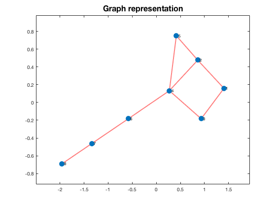
We define now a connected and bidirected graph G. Let E be the edges of the graph. We will define this set as a 2-column matrix and then we create the graph G.
E = [1, 2; 1, 3; 2, 4; 2, 5; 3, 4; 4, 5; 4, 6; 6, 7; 7, 8];
E = table(E,'VariableNames',{'EndNodes'});
G = graph(E);
This is our graph
plot(G, 'LineWidth', 2, 'EdgeColor', 'r', 'MarkerSize', 10)
title('Graph representation', 'FontSize', 16)
N is the size of the graph, that is to say, the number of nodes.
We compute the number of neighbours of each node
connectivities = degree(G);
We check whether the graph is connected or not, if not, we must choose a different graph.
if max(conncomp(G)) > 1
    print('Generate a new graph')
end
In this example the considered graph is connected.
We compute the Perron matrix of $G$.
P = eye(N) - gamma * laplacian(G);
We can see that the system tends to reach a consensus, that is to say, if no control is applied to the system, it evolves to a steady state in which all the nodes have the same state.
We define the initial state $x_0$
x_0 = [1, 5, 0, 4, 3, 1, 7, 3]';
The mean of $x_0$ is 3
The states of the nodes will evolve to the mean of the states at the initial time. We let the system evolve for 150 iterations.
itmax = 150;
x = zeros(N, itmax + 1);
x(:,1) = x_0;
for k = 1:itmax
    x(:,k + 1) = P * x(:,k);
end
clf
hold on
for k = 1:N
    plot(0:itmax,x(k,:),'LineWidth',2)
end
legend('Node 1','Node 2','Node 3','Node 4','Node 5','Node 6','Node 7','Node 8')
title('Graph evolution without control','FontSize',16)
xlabel('Iterations','FontSize',16)
ylabel('States of the nodes','FontSize',16)
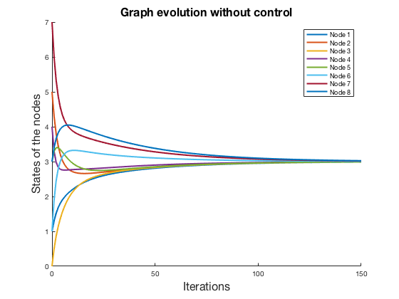
As stated before, we can see in this figure that the system naturally reaches consensus.
Recall that the system dynamics can be written as
for any $k =0,1,…$.
We want to find a control $u$ such that the system stabilizes to the zero state.
We proceed to define matrices B and C:
B = eye(N);
C = eye(N);
%% We can check whether the system is controllable
if rank(ctrb(P,B)) < N
    print('it is not controllable!')
end
%% In this case, it is controllable.
We choose the matrices $Q$ and $R$ by using Bryson and Ho’s criterium.
Q_diag = 1 / max(x_0.^2) * ones(1, N);
R_diag = 1 / 5^2 * ones(1, N);
Q = diag(Q_diag);
R = diag(R_diag);
We can use now the function dlqr (discrete linear quadratic regulator) to find the feedback control $u = -K_{f} x[k]$ that minimizes the functional $J(x,u)$.
[Kf, ~] = dlqr(P, B, Q, R);
Now we can stabilize the system by using the feedback control that we have just computed
itmax = 20;
x = zeros(N, itmax + 1);
x(:,1) = x_0;
for k = 1:itmax
    x(:,k + 1) = (P - B * Kf) * x(:,k);
end
clf
hold on

for k = 1:N
    plot(0:itmax,x(k,:),'LineWidth',2)
end
legend('Node 1','Node 2','Node 3','Node 4','Node 5','Node 6','Node 7','Node 8')
title('Graph stabilization','FontSize',16)
xlabel('Iterations','FontSize',16)
ylabel('States of the nodes','FontSize',16)
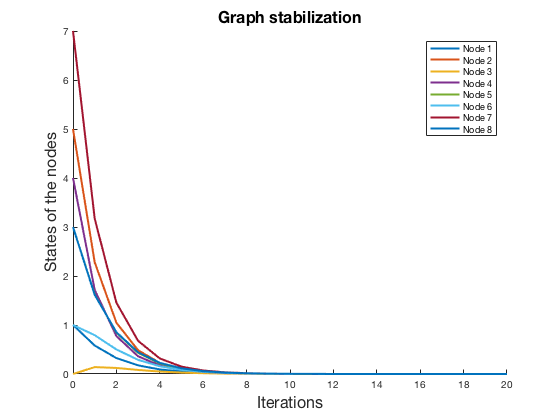
We can see that the system is stabilized fast. One can tune the stabilization speed by choosing matrices $Q$ and $R$ in a smart way.
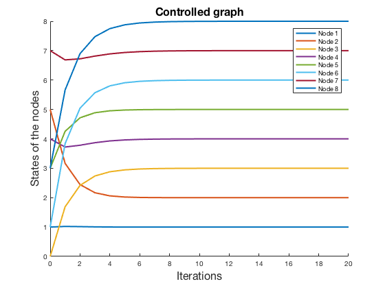
Now, we are about to add a reference term to the control to drive the system to a desired state. For instance, we can drive the system into the reference state
We add a reference term to the control that is proportional to the reference r, $u[k] = -K_{f}x[k] + K_{r}r$. We can use linear algebra to compute the matrix $K_{r}$ in terms of the system matrices.
Kr = -(C * (P - B * Kf - eye(N))^(-1) * B)^(-1);
We drive the system to the reference state.
itmax = 20;
x = zeros(N, itmax + 1);
x(:,1) = x_0;
for k = 1:itmax
    x(:,k + 1) = (P - B * Kf) * x(:,k) + B * Kr * r;
end
clf
hold on
for k = 1:N
    plot(0:itmax,x(k,:),'LineWidth',2)
end
legend('Node 1','Node 2','Node 3','Node 4','Node 5','Node 6','Node 7','Node 8')
title('Controlled graph','FontSize',16)
xlabel('Iterations','FontSize',16)
ylabel('States of the nodes','FontSize',16)
Assume now that we can control only the node 1 and we want to drive the node 8 to the reference state r = 1. Can we do it? Let’s see.
B = zeros(N, 1);
B(1) = 1;
C = zeros(1, N);
C(8) = 1;
if rank(ctrb(P,B)) < N
    print('it is not controllable!')
end
It is controllable.
Q_diag = 1 / max(x_0.^2) * ones(1, N);
R_diag = 1 / 5^2;
Q = diag(Q_diag);
R = diag(R_diag);
[Kf, ~] = dlqr(P, B, Q, R);
Kr = -(C * (P - B * Kf - eye(N))^(-1) * B)^(-1);
r = 1;
itmax = 200;
x = zeros(N, itmax + 1);
x(:,1) = x_0;
for k = 1:itmax
    x(:,k + 1) = (P - B * Kf) * x(:,k) + B * Kr * r;
end
clf
hold on
for k = 1:N
    plot(0:itmax,x(k,:),'LineWidth',2)
end
legend('Node 1','Node 2','Node 3','Node 4','Node 5','Node 6','Node 7','Node 8')
title('Driving node 8 to the state 1','FontSize',16)
xlabel('Iterations','FontSize',16)
ylabel('States of the nodes','FontSize',16)
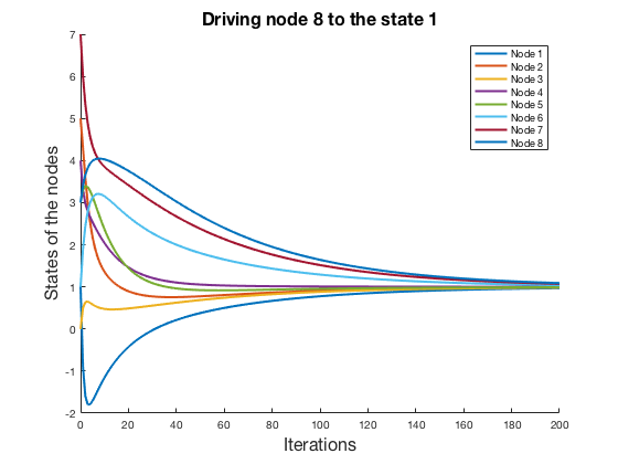
As we can see, the node 8 is driven to the state 1 by achieving consensus in all the states of the graph.
References
[1]: R. Olfati-Saber, J. A. Fax, and R. M. Murray, "Consensus and cooperation in networked multi-agent systems". Proc. IEEE. vol. 95, pp. 215–233, Jan. 2007.
[2]: K. J. Åström, and R. M. Murray, "Feedback Systems: An Introduction for Scientists and Engineers". Princeton University Press, 2008, Princeton, NJ.