Download Code
In [2], we analyzed the controllablity properties under non-negative control and state constraints of the following heat-like equation involving the fractional Laplacian on $(-1,1)$
In \ref{frac_heat}, $\omega\subset (-1,1)$ is the control region in which the distributed control $u$ acts. Moreover, we denote by $(-d_x^2)^s$ the fractional Laplace operator defined, for all $s\in(0,1)$, as the following singular integral
with $c_s$ an explicit normalization constant given by
Gamma being the usual Euler Gamma function.
The main result we established are the following results:
-
For any $s>1/2$, there exists $T>0$ such that the fractional heat equation \ref{frac_heat} is controllable to positive trajectories by means of a non-negative control $u\in L^\infty(\omega\times(0,T))$. Moreover, if the initial datum $z_0\geq 0$ is non-negative, we also have $z(x,t)\geq 0$ for every $(x,t)\in (-1,1)\times (0,T)$.
-
If we define the minimal controllability time by
we have $T_{min}>0$.
- For $T = T_{min}$, there exists a non-negative control $u\in \mathcal M(\omega\times(0,T_{min}))$, the space of Radon measures
on $\omega\times(0,T_{min})$, such that the corresponding solution $z$ of \ref{frac_heat} satisfies $z(x,T) = \widehat{z}(x,T)$ a.e.
in $(-1,1)$.
These results extend to the fractional case the ones previously obtained by our team in the context of the linear and semi-linear heat equation (see our previous entries in the DyCon Blog, WP3_P0001 and WP3_P0002).
In this post, we present some numerical development in order to find the minimal controllability time for the discretized
fractional heat equation with non-negative control constraint and to confirm our theoretical results.
In particular, we will consider the problem of steering the initial datum
to the target trajectroy $\widehat{z}$ solution of \ref{frac_heat} with initial datum
and right-hand side $\widehat{u}\equiv 1$.
We choose $s=0.8$ and $\omega=(-0.3,0.8)\subset (-1,1)$ as the control region. The approximation of the minimal controllability time is obtained by solving the following constrained minimization problem.
subject to
To solve this problem numerically, we employ the expert interior-point optimization routine IpOpt combined with automatic differentiation and the modeling language AMPL. The interest of using AMPL together with IpOpt is that the gradient of the cost function and the constraints is automatically generated. Solving problems with IpOpt and AMPL can be made online through the NEOS solvers.
To perform our simulations, we apply a FE method for the space discretization of the fractional Laplacian (see [1]) on a uniform space-grid
with $N_x=20$ . Moreover, we use an explicit Euler scheme for the time integration on the time-grid
with $N_t$ satisfying the Courant-Friedrich-Lewy condition. In particular, we choose here $N_t=100$.
The AMPL code for solving this minimation problem is included below. In it, the matrices defining the dynamics are computed through specific functions implemented in Matlab and are given as parameters.
It is important to remark that we are interested in the controllability to the trajectory $\widehat{z}(\cdot,T)$ but, at the same time, $T$ is a variable in our code since it is the cost functional we aim to minimize. In view of that, our final target changes during the minimization process. Nevertheless this issue can be bypassed by taking advance of the linear nature of our equation and solving the traslated constrained minimization problem consisting in finding the minimial time for steering the inital datum $z_0-\widehat{z}_0$ by employing a control $u\geq\widehat{u}$ ($\widehat{z}_0$ and $\widehat{u}$ are the same given above).
# Minimal time for the constrained controllability of the fractional heat equation.

# 1: define the parameters

param Nx = 20;               # number of spatial discretization points

param Nt = 100;              # number of time discretization points

param y0 {1..Nx};            # initial condition

param y1 = 0;                # target

param dx = 2/Nx;             # Space step

param C = 1;                 # Bound on the controls

param A {1..Nx,1..Nx};       # Stiffness or rigidity matrix

param B {1..Nx,1..Nx};       # Control matrix

param M {1..Nx,1..Nx};       # Mass matrix

# 2: define the variables

var y {j in 0..Nt, i in 1..Nx};       # State
var u {j in 0..Nt, i in 1..Nx}>=-C;   # Control
var T >=0;                            # Time horizon
var dt = T/Nt;                        # Time step

# 3: define the data

data;

# Initial datum

param y0: 1 2 3 4 5 6 7 8 9 10 11 12 13 14 15 16 17 18 19 20 :=
1 -0.000000 -0.905270 -1.785847 -2.617711 -3.378170 -4.046482 -4.604416 -5.036753 -5.331701 -5.481215 -5.481215 -5.331701 -5.036753 -4.604416 -4.046482 -3.378170 -2.617711 -1.785847 -0.905270 -0.000000;

# Stiffness or rigidity matrix A

param A: 1 2 3 4 5 6 7 8 9 10 11 12 13 14 15 16 17 18 19 20 :=
1 -5.551728 2.242487 0.359689 0.077115 0.033148 0.017829 0.010871 0.007193 0.005044 0.003694 0.002798 0.002178 0.001733 0.001405 0.001158 0.000966 0.000816 0.000697 0.000600 0.000521
...
20 0.000521 0.000600 0.000697 0.000816 0.000966 0.001158 0.001405 0.001733 0.002178 0.002798 0.003694 0.005044 0.007193 0.010871 0.017829 0.033148 0.077115 0.359689 2.242487 -5.551728;
# Control matrix B

param B: 1 2 3 4 5 6 7 8 9 10 11 12 13 14 15 16 17 18 19 20 :=
1 0.000000 0.000000 0.000000 0.000000 0.000000 0.000000 0.000000 0.000000 0.000000 0.000000 0.000000 0.000000 0.000000 0.000000 0.000000 0.000000 0.000000 0.000000 0.000000 0.000000
...
20 0.000000 0.000000 0.000000 0.000000 0.000000 0.000000 0.000000 0.000000 0.000000 0.000000 0.000000 0.000000 0.000000 0.000000 0.000000 0.000000 0.000000 0.000000 0.000000 0.000000;
# Mass matrix M

param M: 1 2 3 4 5 6 7 8 9 10 11 12 13 14 15 16 17 18 19 20 :=
1 0.070175 0.017544 0.000000 0.000000 0.000000 0.000000 0.000000 0.000000 0.000000 0.000000 0.000000 0.000000 0.000000 0.000000 0.000000 0.000000 0.000000 0.000000 0.000000 0.000000
...
20 0.000000 0.000000 0.000000 0.000000 0.000000 0.000000 0.000000 0.000000 0.000000 0.000000 0.000000 0.000000 0.000000 0.000000 0.000000 0.000000 0.000000 0.000000 0.017544 0.070175;
# 4: define the cost functional to minimize

minimize cost: T;

# 5: define the constraints

# 5.a: dynamics y' = Ay + Bu, implemented through an Explicit Euler method.

subject to y_dyn {j in 1..Nt, i in 2..Nx-1}:
sum {l in 1..Nx} M[i,l]*y[j,l] = sum {l in 1..Nx}M[i,l]*y[j-1,l] + dt*sum {l in 1..Nx}(A[i,l]*y[j-1,l] + B[i,l]*u[j-1,l]);

# 5.b: homogeneous Dirichlet boundary conditions in -1 and 1.

subject to left_boundary  {j in 0..Nt}: y[j,1] = 0;
subject to right_boundary {j in 0..Nt}: y[j,Nx] = 0;

# 5.c: initial condition.

subject to y_init {i in 1..Nx}: y[0,i] = y0[i];

# 5.d: target.

subject to y_end1 {i in 1..Nx}: y[Nt,i] = y1;

# 6: solve the problem with IpOpt

option solver ipopt;
option ipopt_options "max_iter=100000 linear_solver=mumps hessian_approximation=exact halt_on_ampl_error yes";
solve;

# 7: print the results.

printf: "T  = %24.16e\n", T;
printf: "Nx = %d\n", Nx;
printf: "Nt = %d\n", Nt;
printf {j in 0..Nt, i in 1..Nx}: " %24.16e\n", y[j,i];
printf {j in 0..Nt, i in 1..Nx}: " %24.16e\n", u[j,i];

end;
Once the minimization is concluded, we save the results in a file “data.txt” and we use Matlab to reshape the solution and the control so to obtain two $N_x\times(N_t+1)$ matrices for the plots.
This can be done through the following script:
close all
% Read the data from the external file data.txt

fid= fopen('data.txt','r');
C = fscanf(fid,'%f',Inf);
T = C(1);
Nx = C(2);
Nt = C(3);
y = C(4:(Nt+1)*Nx+3);
u = C((Nt+1)*Nx+4:end);
fclose(fid);

% Reshape the state y and the control u into two Nx times Nt+1 matrices
y = reshape(y,Nx,Nt+1);
u = reshape(u,Nx,Nt+1);
From the reshaped solution and control, we can generate the plots. For instance, the m-file plot_control.m is the one generating Figure 2 below.
The minimal time that we obtain from our minimization process is $T_{min}\simeq 0,2101$. Our simulations show that in this time horizon the fractional heat equation \ref{frac_heat} is controllable from the initial datum $z_0$ to the desired trajectory $\widehat{z}(\cdot,T)$ by maintaining the positivity of the solution (as it is expected since the initial datum is positive in $(-1,1)$, see Figure 1).

Figure 1. Controllability of the fractional heat equation \ref{frac_heat}in the minimal time $T_{min}=0.2101$.
Moreover, as it is observed also in Figure 2, the control has an impulsional behavior.
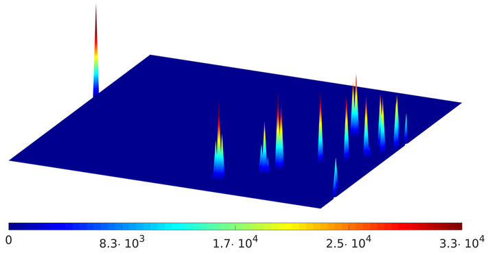
Figure 2. Minimal-time control. In the $(t,x)$ plane in blue the time $t$ varies from $t = 0$ (left) to $t = T_{min}$ (right).
This behavior of the control is not surprising. Indeed, as it was already observed in our previous works [3,4], the minimal-time controls are expected to be atomic measures, in particular linear combinations of Dirac deltas. Our simulations are thus consistent with the aforementioned papers.
The impulsional behavior of the control is then lost when extending the time horizon beyond $T_{min}$. This is shown in Figure 3, in which we display the behavior of the control steering the solution of the fractional heat equation \ref{frac_heat} from the initial datum $z_0$ to the target $\widehat{z}(\cdot,T)$ in the time horizon $T=0.4$.
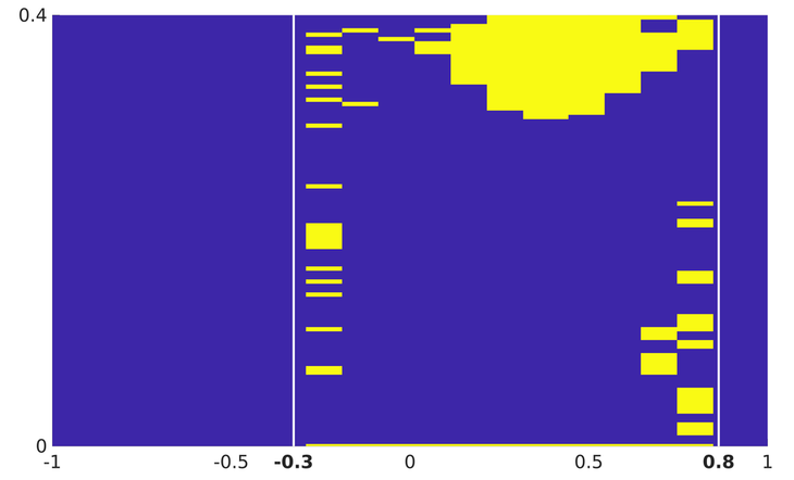
Figure 3. Behavior of the control in time $T = 0.4$. The white lines delimit the control region $\omega = (-0.3, 0.8)$. The regions in which the control is active are marked in yellow. The atomic nature is lost.
This control has been computed by employing once again IpOpt for solving the following minimization problem:
subject to
As we can observe, the action of this control is now more distributed in $\omega$. Neverthelss, in accordance with our theoretical results, the equation is still controllable in the prescribed time horizon (see Figure 4)
Figure 4. Controllability of the fractional heat equation \ref{frac_heat}in time $T = 0.4$. The atomic behavior of the control is lost.
Finally, we consider the case of a time horizon $T<T_{min}$, in which constrained controllability is expected to fail. This time, we employ a classical conjugate gradient method implemented in the DyCon Computational Toolbox for solving the above optimization problem.
As before, we apply a FE method for the space discretization of the fractional Laplacian on a uniform space-grid with $N_x=20$ points and we use an explicit Euler scheme for the time integration on a time-grid with $N_t=100$ points. Furthermore, we choose a time horizon $T=0.15$, which is below the minimal controllability time $T_{min}$.
Our simulation then show that the solution of \ref{frac_heat} fails to be controlled. In fact, Figure 5 shows that the state computed by employing the tools of the DyCon Computational Toolbox does not totally match the desired target in the time horizon prescribed.
Figure 5. Evolution in the time interval $(0,0.15)$ of the solution of \ref{frac_heat} with $s = 0.8$ under the positivity control constraint $u\geq 0$. The equation is not controllable.
References
[1] U. Biccari and V. Hernández-Santamarı́a, Controllability of a one-dimensional fractional heat equation: theoretical and
numerical aspects. IMA J. Math. Control. Inf, to appear, 2018.
[2] U. Biccari, M. Warma and E. Zuazua, Controllability of the one-dimensional fractional heat equation under positivity constraints. Submitted.
[3] J. Loheac, E. Trélat, and E. Zuazua, Minimal controllability time for the heat equation under unilateral state or control
constraints. Math. Models Methods Appl. Sci., Vol. 27, No. 9 (2017), pp 1587-1644.
[4] D. Pighin and E. Zuazua, Controllability under positivity constraints of semilinear heat equations. Math. Control. Relat.
Fields, Vol. 8, No. 3,4 (2018), pp. 935-964.