Download Code
This code needs the installation of CasADi 3.4.5: https://web.casadi.org/get/
The objectives of this post are twofold, one is to introduce CasADi (with IpOpt) to simulate optimal control problem, and the other is to introduce the concept of the structural controllability, as an example, for the 2D heat equation.
Controllability of the 2D heat equation
In this post, we simulate structural controllability for the two-dimensional heat equation. First, we start with the finite difference scheme of the 2D Heat equation and the control on one boundary of the square domain $[0,1]^2$.
A similar problem has been treated in another DyCon Blog post using AMPL and IpOpt, which deals with the one-dimensional fractional heat equation under positivity constraints. Here we use CasADi and IpOpt in Matlab language.
We will consider the problem of steering the initial datum:
to the final target $(1.5 \cdot \bar z_{i,j}(T))$, where $\bar z_{i,j}(T)$ is a reference solution from $z^0_{i,j}$ without control.
Parameters for the problem:
N_size = 4; %% Space discretization for 1D
Nx = N_size^2; %% Space discretization for 2D
Nt = 20; %% Time discretization
T = 0.1; %% Final time

%% Discretization of the Space
xline_ = linspace(0,1,N_size+2);
[xmsf,ymsf] = meshgrid(xline_,xline_);
xline = xline_(2:end-1);
[xms,yms]   = meshgrid(xline,xline);

dx = xline(2) - xline(1);

%% Initial data
Y0_2d = zeros(N_size);
for i=1:N_size
    for j=1:N_size
        Y0_2d(i,j) = sin(xline(i)*pi)*sin(xline(j)*pi);
    end
end
Y0 = Y0_2d(:);


%% Definition of the dynamics : Y' = AY+BU
B = zeros(N_size^2,N_size); B(1:N_size,1:N_size) = eye(N_size); %% control for i=1,...,N_size.

A1_mat = ones(N_size,1);
A2_mat = spdiags([A1_mat -2*A1_mat A1_mat], [-1 0 1], N_size,N_size);
I_mat  = speye(N_size);
A_mat  = kron(I_mat,A2_mat)+kron(A2_mat,I_mat);

A = A_mat; %% A: Discrete Laplacian in 2D with uniform squared mesh

%% Discretization of the time : we need to check CFL condition to change 'Nt'.
tline = linspace(0,T,Nt+1); %%uniform time mesh

dt = tline(2)-tline(1);
The interactions between nodes (grid points) can be displayed as follows:
options_plot_graphs = {'LineWidth',2,'DisplayName','off','NodeColor','r','ArrowSize',9,'MarkerSize',7,'NodeLabel',{}};
p = plot(digraph(A),'XData',xms(:)','YData',yms(:)',options_plot_graphs{:});
hold on
plot(xms(:,1),yms(:,1),'b.','MarkerSize',30) %% Blue dots are controlled nodes
xlabel('x-axis')
ylabel('y-axis')
grid on
for i=1:N_size.^2
    text(p.XData(i)+0.01, p.YData(i)+0.02, num2str(i), 'FontSize', 20);
end
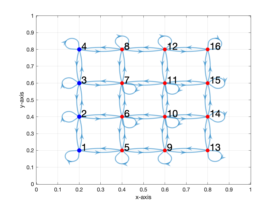
Fig 1. The interaction network of 'A_mat'. The controlled nodes are colored blue.
Now we may simulate the reference trajectory without control.
%% Simulation of the uncontrolled trajectory
M = eye(Nx) - 0.5*dt/dx.^2*A;
L = eye(Nx) + 0.5*dt/dx.^2*A;
P = 0.5*dt*B;

Y = zeros(Nx,Nt+1);

Y(:,1) = Y0;
for k=1:Nt %% loop over time intervals
   %% Crank-Nicolson method without control
   Y(:,k+1) = M\L*Y(:,k);
end
YT = Y(:,Nt+1);

ratio = 1.5;
Y1 = ratio*YT; %% Target data

clf
Z = reshape(Y(:,1),N_size,N_size);
Z = [zeros(1,N_size+2) ; zeros(N_size,1), Z, zeros(N_size,1) ; zeros(1,N_size+2)];
isurf = surf(xmsf,ymsf,Z,'FaceAlpha',0.3);
isurf.CData = isurf.CData*0 + 10;
hold on
Z = reshape(Y(:,end),N_size,N_size);
Z = [zeros(1,N_size+2) ; zeros(N_size,1), Z, zeros(N_size,1) ; zeros(1,N_size+2)];
jsurf = surf(xmsf,ymsf,Z,'FaceAlpha',0.7);
jsurf.CData = jsurf.CData*0 + 1;
jsurf.Parent.Color = 'none';
lightangle(10,10)
legend({'Initial Condition','Final Data'})
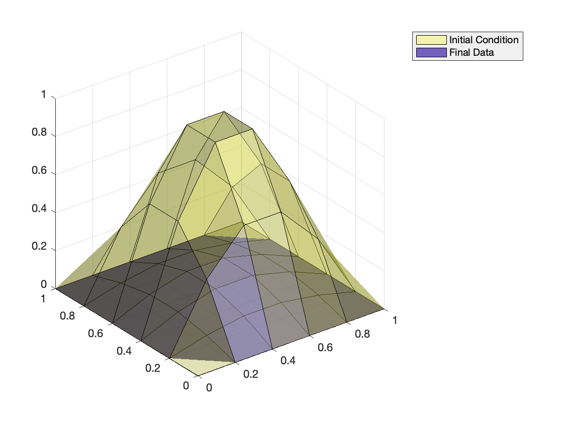
Fig 2. The initial condition and the final data of uncontrolled dynamics.
Optimization problem
From now on, we use CasADi to consider an exact control problem.
opti = casadi.Opti();  %% CasADi function

%% ---- Input variables ---------
X = opti.variable(Nx,Nt+1); %% state trajectory
U = opti.variable(N_size,Nt+1);   %% control

%% ---- Dynamic constraints --------
for k=1:Nt %% loop over control intervals
   %% Crank-Nicolson method : this helps us to boost the optimization
   opti.subject_to(M*X(:,k+1)== L*X(:,k) + 0.5*P*(U(:,k)+U(:,k+1)));
end

%% ---- State constraints --------
opti.subject_to(X(:,1)==Y0);
opti.subject_to(X(:,Nt+1)==Y1);

%% ---- Optimization objective  ----------
Cost = (dx*sum(sum(U.^2))*(T/Nt));
opti.minimize(Cost); %% minimizing L2 over time

%% ---- initial guesses for solver ---
opti.set_initial(X, Y);
opti.set_initial(U, 0);

%% ---- solve NLP              ------
p_opts = struct('expand',true);
s_opts = struct('max_iter',10000); %% iteration limitation

opti.solver('ipopt',p_opts,s_opts); %% set numerical backend
tic
sol = opti.solve();   %% actual solve
toc
This is Ipopt version 3.12.3, running with linear solver mumps.
NOTE: Other linear solvers might be more efficient (see Ipopt documentation).

Number of nonzeros in equality constraint Jacobian...:     2752
Number of nonzeros in inequality constraint Jacobian.:        0
Number of nonzeros in Lagrangian Hessian.............:       84

Total number of variables............................:      420
                     variables with only lower bounds:        0
                variables with lower and upper bounds:        0
                     variables with only upper bounds:        0
Total number of equality constraints.................:      352
Total number of inequality constraints...............:        0
        inequality constraints with only lower bounds:        0
   inequality constraints with lower and upper bounds:        0
        inequality constraints with only upper bounds:        0

iter    objective    inf_pr   inf_du lg(mu)  ||d||  lg(rg) alpha_du alpha_pr  ls
   0  0.0000000e+00 6.69e-02 0.00e+00  -1.0 0.00e+00    -  0.00e+00 0.00e+00   0
   1  1.6511358e+02 6.66e-16 7.31e-07  -2.5 8.68e+01    -  1.00e+00 1.00e+00h  1
   2  1.6511358e+02 6.66e-16 2.39e-12  -8.6 5.47e-09    -  1.00e+00 1.00e+00h  1

Number of Iterations....: 2

                                   (scaled)                 (unscaled)
Objective...............:   1.6511358437684962e+02    1.6511358437684962e+02
Dual infeasibility......:   2.3874235921539366e-12    2.3874235921539366e-12
Constraint violation....:   6.6613381477509392e-16    6.6613381477509392e-16
Complementarity.........:   0.0000000000000000e+00    0.0000000000000000e+00
Overall NLP error.......:   4.0210221040688533e-13    2.3874235921539366e-12


Number of objective function evaluations             = 3
Number of objective gradient evaluations             = 3
Number of equality constraint evaluations            = 3
Number of inequality constraint evaluations          = 0
Number of equality constraint Jacobian evaluations   = 3
Number of inequality constraint Jacobian evaluations = 0
Number of Lagrangian Hessian evaluations             = 2
Total CPU secs in IPOPT (w/o function evaluations)   =      0.822
Total CPU secs in NLP function evaluations           =      0.000

EXIT: Optimal Solution Found.
               t_proc [s]   t_wall [s]    n_eval
       nlp_f      1.9e-05      1.9e-05         3
       nlp_g     0.000103     0.000105         3
  nlp_grad_f      3.7e-05      3.4e-05         4
  nlp_hess_l      1.4e-05      1.3e-05         2
   nlp_jac_g     0.000185     0.000195         4
      solver         1.09        0.676         1
Elapsed time is 0.757156 seconds.
Post-processing
Sol_x = sol.value(X); %% solved controlled trajectory
Sol_u = sol.value(U); %% solved control function

clf
Z = zeros(N_size+2,N_size+2);
Z(2:end-1,2:end-1) = reshape(Sol_x(:,end),N_size,N_size);
isurf = surf(xmsf,ymsf,Z,'FaceAlpha',0.3);
isurf.CData = isurf.CData*0 + 10;
hold on
Z = zeros(N_size+2,N_size+2);
Z(2:end-1,2:end-1) = reshape(Y(:,end),N_size,N_size);
jsurf = surf(xmsf,ymsf,Z,'FaceAlpha',0.7);
jsurf.CData = jsurf.CData*0 + 1;

Z = zeros(N_size+2,N_size+2);
Z(2:end-1,2:end-1) = ratio*reshape(Y(:,end),N_size,N_size);
plot3(xmsf,ymsf,Z,'k*')

jsurf.Parent.Color = 'none';
lightangle(10,10)

legend({'Controlled final data','Uncontrolled final data','Target'})
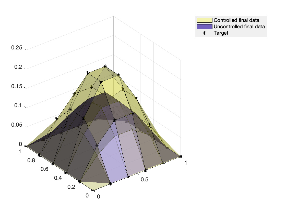
Fig 3. The final data of controlled and uncontrolled dynamics. The controlled data coinside with the target points.
%% Free and controlled dynamics in animation

Result_ref = zeros(N_size+2,N_size+2,Nt+1); %% displaying variable
Result_ref(2:end-1,2:end-1,:) = reshape(Y(:,:),[N_size,N_size,Nt+1]);

Result_con2d = zeros(N_size+2,N_size+2,Nt+1); %% displaying variable
Result_con2d(2:end-1,2:end-1,:) = reshape(Sol_x(:,:),[N_size,N_size,Nt+1]);
%% Free dynamics
fig = figure;
isurf2= surf(ratio*Result_ref(:,:,end),'FaceAlpha',0.3);
isurf2.CData = isurf2.CData*0 + 1;
hold on
isurf = surf(Result_ref(:,:,1),'FaceAlpha',0.7);
isurf.CData = isurf.CData*0 + 10;
title('Free dynamics')
legend('Target','Solution')
zlim([-0.5 1.5])
pause;
for it = 1:Nt+1
   isurf.ZData =  Result_ref(:,:,it);
    pause(0.1)
end
%% Controlled dynamics
clf
fig = figure;
isurf2= surf(ratio*Result_ref(:,:,end),'FaceAlpha',0.3);
isurf2.CData = isurf2.CData*0 + 1;
hold on
isurf = surf(Result_con2d(:,:,1),'FaceAlpha',0.7);
isurf.CData = isurf.CData*0 + 10;
title('Controlled dynamics')
legend('Target','Solution')
zlim([-0.5 1.5])
pause;
for it = 1:Nt+1
   isurf.ZData =  Result_con2d(:,:,it);
    pause(0.1)
end
Fig 4-5. Animations for the free and controlled dynamics. The target surface is also drawn in both dynamics, where free dynamics goes below than the target.
Structural controllability of the 2D heat equation
For the second part, we simulate another linear system to check the structural controllability of the 2D heat equation. It is known that its interacting network is structurally controllable by one sole node.
The following matrix ‘AS_mat’ links the nodes in a line, for example, 1-2-3-6-5-4-7-8-9 for $N=3$, which is a part of interactions in ‘A_mat’:
AC_mat = diag(ones(N_size-1,1),-1);
for j=1:2:N_size-2
    AC_mat = blkdiag(AC_mat,diag(ones(N_size-1,1),1));
    AC_mat(end,end-N_size)=1;
    if N_size==2
        break
    end
    AC_mat = blkdiag(AC_mat,diag(ones(N_size-1,1),-1));
    AC_mat(end-N_size+1,end-2*N_size+1)=1;
end
if length(AC_mat) < (N_size.^2)
    AC_mat = blkdiag(AC_mat,diag(ones(N_size-1,1),1));
    AC_mat(end,end-N_size)=1;
end

AS_mat = (AC_mat + AC_mat') - 2*eye(Nx);

options_plot_graphs = {'LineWidth',2,'DisplayName','off','NodeColor','r','ArrowSize',9,'MarkerSize',7,'NodeLabel',{}};
p = plot(digraph(AS_mat),'XData',xms(:)','YData',yms(:)',options_plot_graphs{:});
xlabel('x-axis');ylabel('y-axis')
hold on
plot(xms(1,1),yms(1,1),'b.','MarkerSize',30) %% Blue dots are controlled nodes
for i=1:N_size.^2
    text(p.XData(i)+0.01, p.YData(i)+0.02, num2str(i), 'FontSize', 20);
end

title('Network')
grid on
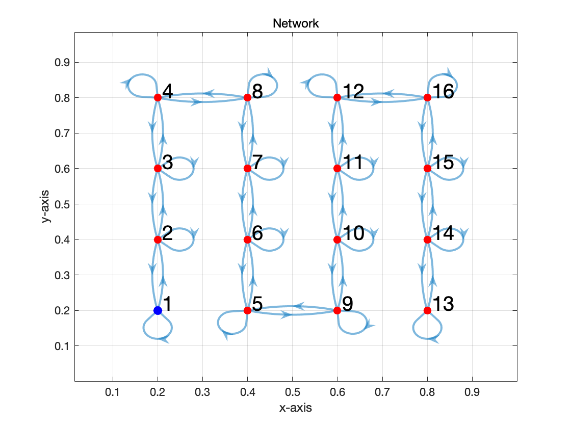
Fig 6. The interaction network of the new matrix 'AS_mat'. The controlled nodes are colored blue.
Since the 1D heat equation is controllable, ‘AS_mat’ is controllable by one node. However, it gets more and more difficult as the number of nodes increases, since it has different scale with the standard 1D heat equation. The length of the 1D domain grows as $N$ since it eventually become space filling curve in $[0,1]^2$.
Note also that ‘AS_mat’ has the nonzero elements in the positions that ‘A_mat’ has. By deleting several interactions of ‘A_mat’, ‘AS_mat’ is now exactly controllable with smaller controlled nodes. This is the idea of the structural controllability in the network system, called ‘network control’.
B = zeros(N_size^2,1); B(1) = 1;
A = N_size.^2*AS_mat;
%% Y' = AY + BU

T = 0.1;
Nt = 30;
tline = linspace(0,T,Nt+1); %%uniform time mesh
dt = tline(2)-tline(1);

%% Simulation of the uncontrolled trajectory
M = eye(Nx) - 0.5*dt/dx.^2*A;
L = eye(Nx) + 0.5*dt/dx.^2*A;
P = 0.5*dt*B;

Y = zeros(Nx,Nt+1);
Y(:,1) = Y0;
for k=1:Nt %% loop over time intervals
   %% Crank-Nicolson method without control
   Y(:,k+1) = M\L*Y(:,k);
end
YT = Y(:,Nt+1);
Y1 = ratio*YT;
Optimization problem in CasADi
opti = casadi.Opti();  %% CasADi function

%% ---- Input variables ---------
X = opti.variable(Nx,Nt+1); %% state trajectory
U = opti.variable(1,Nt+1);   %% control

%% ---- Dynamic constraints --------
for k=1:Nt %% loop over control intervals
   %% Crank-Nicolson method
   opti.subject_to(M*X(:,k+1)== L*X(:,k) + P*(U(:,k)+U(:,k+1)));
end

%% ---- State constraints --------
opti.subject_to(X(:,1)==Y0);
opti.subject_to(X(:,Nt+1)==Y1);

%% ---- Optimization objective  ----------
Cost = (sum(U.^2)*(T/Nt)); %%1e3*dx^2*sum(sum((X(:,Nt+1)-Y1).^2))+;
opti.minimize(Cost); %% minimizing L2 at the final time

%% ---- Initial guess ----
opti.set_initial(X, Y);
opti.set_initial(U, 0);

%% ---- solve NLP              ------
p_opts = struct('expand',true);
s_opts = struct('max_iter',1e5); %% cut down the algorithm at the 1000-th iteration.
opti.solver('ipopt',p_opts,s_opts); %% set numerical backend
tic
sol = opti.solve();   %% actual solve
toc
This is Ipopt version 3.12.3, running with linear solver mumps.
NOTE: Other linear solvers might be more efficient (see Ipopt documentation).

Number of nonzeros in equality constraint Jacobian...:     2852
Number of nonzeros in inequality constraint Jacobian.:        0
Number of nonzeros in Lagrangian Hessian.............:       31

Total number of variables............................:      527
                     variables with only lower bounds:        0
                variables with lower and upper bounds:        0
                     variables with only upper bounds:        0
Total number of equality constraints.................:      512
Total number of inequality constraints...............:        0
        inequality constraints with only lower bounds:        0
   inequality constraints with lower and upper bounds:        0
        inequality constraints with only upper bounds:        0

iter    objective    inf_pr   inf_du lg(mu)  ||d||  lg(rg) alpha_du alpha_pr  ls
   0  0.0000000e+00 1.04e-01 0.00e+00  -1.0 0.00e+00    -  0.00e+00 0.00e+00   0
   1  2.9522421e+04 1.33e-15 6.25e-02  -2.5 1.08e+03    -  1.00e+00 1.00e+00h  1

Number of Iterations....: 1

                                   (scaled)                 (unscaled)
Objective...............:   2.9522420557910038e+04    2.9522420557910038e+04
Dual infeasibility......:   6.2500000000000000e-02    6.2500000000000000e-02
Constraint violation....:   1.3322676295501878e-15    1.3322676295501878e-15
Complementarity.........:   0.0000000000000000e+00    0.0000000000000000e+00
Overall NLP error.......:   1.4002321948103652e-12    6.2500000000000000e-02


Number of objective function evaluations             = 2
Number of objective gradient evaluations             = 2
Number of equality constraint evaluations            = 2
Number of inequality constraint evaluations          = 0
Number of equality constraint Jacobian evaluations   = 2
Number of inequality constraint Jacobian evaluations = 0
Number of Lagrangian Hessian evaluations             = 1
Total CPU secs in IPOPT (w/o function evaluations)   =      0.516
Total CPU secs in NLP function evaluations           =      0.000

EXIT: Optimal Solution Found.
               t_proc [s]   t_wall [s]    n_eval
       nlp_f      6.2e-05      1.4e-05         2
       nlp_g     0.000212       0.0001         2
  nlp_grad_f      4.3e-05      2.9e-05         3
  nlp_hess_l      3.2e-05      3.3e-05         1
   nlp_jac_g     0.000147     0.000148         3
      solver        0.668        0.573         1
Elapsed time is 0.638270 seconds.
Post-processing
Sol_x = sol.value(X); %% solved controlled trajectory
Sol_u = sol.value(U); %% solved control
%%Sol_x = opti.debug.value(X);
%%Sol_u = opti.debug.value(U); %% final data if algorithm stops with error

%%
clf
Z = zeros(N_size+2,N_size+2);
Z(2:end-1,2:end-1) = reshape(Sol_x(:,end),N_size,N_size);
isurf = surf(xmsf,ymsf,Z,'FaceAlpha',0.3);
isurf.CData = isurf.CData*0 + 10;
hold on
Z = zeros(N_size+2,N_size+2);
Z(2:end-1,2:end-1) = reshape(Y(:,end),N_size,N_size);
jsurf = surf(xmsf,ymsf,Z,'FaceAlpha',0.7);
jsurf.CData = jsurf.CData*0 + 1;

Z = zeros(N_size+2,N_size+2);
Z(2:end-1,2:end-1) = ratio*reshape(Y(:,end),N_size,N_size);
plot3(xmsf,ymsf,Z,'k*')

jsurf.Parent.Color = 'none';
lightangle(10,10)

legend({'Controlled final data','Uncontrolled final data','Target'})
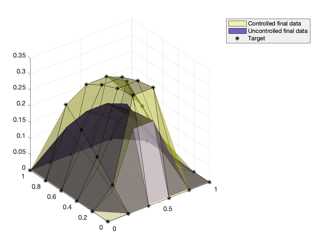
Fig 7. The initial condition and the final data of uncontrolled dynamics. It has a different structure compared to Fig 2.
%% Free and controlled dynamics in animation

Result_ref = zeros(N_size+2,N_size+2,Nt+1); %% displaying variable
Result_ref(2:end-1,2:end-1,:) = reshape(Y(:,:),[N_size,N_size,Nt+1]);

Result_con2d = zeros(N_size+2,N_size+2,Nt+1); %% displaying variable
Result_con2d(2:end-1,2:end-1,:) = reshape(Sol_x(:,:),[N_size,N_size,Nt+1]);

fig = figure;
isurf2= surf(ratio*Result_ref(:,:,end),'FaceAlpha',0.3);
isurf2.CData = isurf2.CData*0 + 1;
hold on
isurf = surf(Result_ref(:,:,1),'FaceAlpha',0.7);
isurf.CData = isurf.CData*0 + 10;
title('Free dynamics')
legend('Target','Solution')
zlim([-0.5 1.5])
pause;
for it = 1:Nt+1
   isurf.ZData =  Result_ref(:,:,it);
    pause(0.1)
end

%%
clf

fig = figure;
isurf2= surf(ratio*Result_ref(:,:,end),'FaceAlpha',0.3);
isurf2.CData = isurf2.CData*0 + 1;
hold on
isurf = surf(Result_con2d(:,:,1),'FaceAlpha',0.7);
isurf.CData = isurf.CData*0 + 10;
title('Controlled dynamics')
legend('Target','Solution')
zlim([-0.5 1.5])
pause;
for it = 1:Nt+1
   isurf.ZData =  Result_con2d(:,:,it);
    pause(0.1)
end
Fig 8-9. Animations for the free and controlled dynamics. The target surface is also drawn in both dynamics, where free dynamics goes below than the target.