A sample result
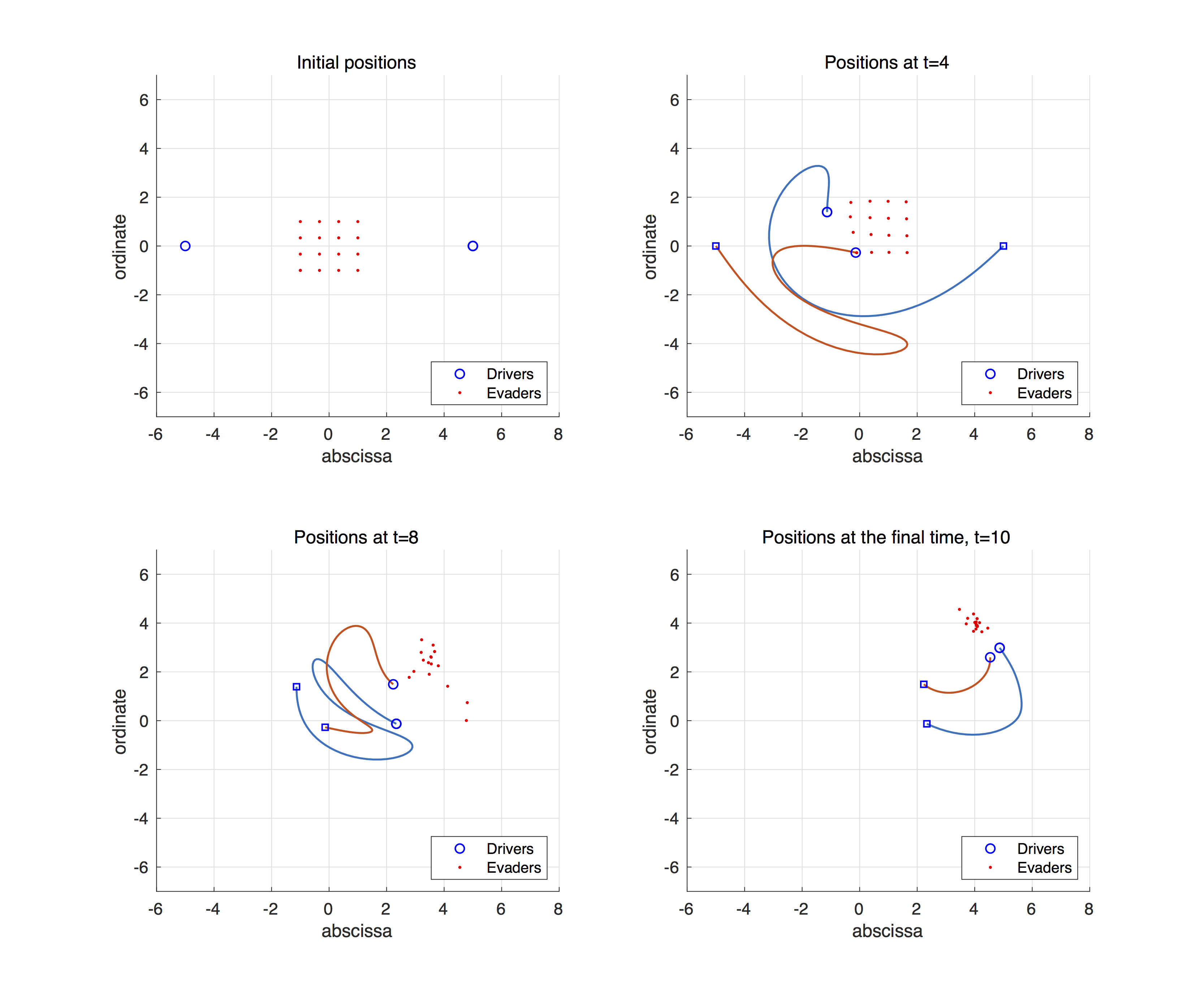
This video describes an optimal control steering red dots(evaders) to the position $(4,4)$, which is calculated by IpOpt with AMPL. See the post explaining IpOpt and AMPL for detailed description.
The guidance-by-repulsion model
Let $u_{ei}$ and $u_{dj}$ be the positions of the evaders $(i=1,\ldots,N)$ and drivers $(j=1,\ldots,M)$, respectively, in ${\mathbb R}^2$. We consider the following ODE system:
where $\kappa_j(t)$ is the control interface and the interaction functions are given by
In the dynamics, the evaders always get forced from all of the drivers, while the drivers wants to keep a stable distance ($f_d(1)-f_e(1)=0$). By choosing proper $\kappa_j(t)$, we wants to steer the evaders into a predetermined region.
The objective of the control is given by the cost function with the fixed final time $t_f>0$,
where $\delta_1$ is a regularization coefficient, $0.1$ in this post.
AMPL code for solving the optimal control problem
Let us explain an AMPL code step by step. First, we need to set relative parameters.
# GBR_fixedtime.mod

# This file solves the Guidance-by-repulsion model with 2 drivers and 16 evaders to

# the target point [4;4] in a fixed final time T=10.

# Define the parameters of the problem

param pi      = 3.141592653589793238462643;

param Nt      = 100;      # number of discretized points in time

param M_sqrt  = 4;        # sqrt of Number of evaders

param M_e     = M_sqrt^2; # Number of evaders

param M_d     = 2;        # Number of drivers

param T       = 10;

param M_kappa = 5;        # Bound on the control

# Target point

param uf1 = 4;
param uf2 = 4;
For the initial condition, we use uniform distribution of evaders in a square $[-1,1]\times[-1,1]$, and the drivers are in a circle with radius $5$.
# Initial values

param ue_zero {k in 1..M_e, j in 1..2};
for {k1 in 1..M_sqrt, k2 in 1..M_sqrt, j in 1..2} {
	let ue_zero[M_sqrt*(k1-1)+k2,1] := ((k1-1)/(M_sqrt-1))*2-1;
	let ue_zero[M_sqrt*(k1-1)+k2,2] := ((k2-1)/(M_sqrt-1))*2-1;
}
param ud_zero {l in 1..M_d, j in 1..2};
for {l in 1..M_d, j in 1..2} {
	let ud_zero[l,1] := 5*cos(2*pi/M_d*(l-1));
	let ud_zero[l,2] := 5*sin(2*pi/M_d*(l-1));
}

# State variables

var ue {k in 1..M_e, i in 0..Nt, j in 1..2};
var ve {k in 1..M_e, i in 0..Nt, j in 1..2};
var ud {l in 1..M_d, i in 0..Nt, j in 1..2};
var vd {l in 1..M_d, i in 0..Nt, j in 1..2};
var uec {i in 0..Nt, j in 1..2} = 1/M_e*(sum {k in 1..M_e} (ue[k,i,j]));

# initialize

subject to ue_init {k in 1..M_e, j in 1..2} : ue[k,0,j] = ue_zero[k,j];
subject to ud_init {l in 1..M_d, j in 1..2} : ud[l,0,j] = ud_zero[l,j];
subject to vd_init {k in 1..M_e, j in 1..2} : ve[k,0,j] = 0;
subject to ve_init {l in 1..M_d, j in 1..2} : vd[l,0,j] = 0;
let {k in 1..M_e, i in 0..Nt, j in 1..2} ue[k,i,j] := ue_zero[k,j];
let {l in 1..M_d, i in 0..Nt, j in 1..2} ud[l,i,j] := ud_zero[l,j];
let {k in 1..M_e, i in 0..Nt, j in 1..2} ve[k,i,j] := 0;
let {l in 1..M_d, i in 0..Nt, j in 1..2} vd[l,i,j] := 0;
For the initial guess, we also put the initial data for the whole timeline. If we don’t specify this, then the default values are zero, which can make redundant errors or iterations.
Now, we define the controls and cost.
# The control function

var kappa {l in 1..M_d, i in 0..Nt}, default 2.8;
subject to kappa_bounds {l in 1..M_d, i in 0..Nt} : -M_kappa <= kappa[l,i] <= M_kappa;
# initial guess on control

let {l in 1..M_d, i in 0..Nt} kappa[l,i] := 2.8;

# The cost function

minimize cost:
 1/M_e*(sum {k in 1..M_e} ((ue[k,Nt+1,1]-uf1)^2+(ue[k,Nt+1,2]-uf2)^2)) + 0.1/M_d/(Nt+1)*( sum {l in 1..M_d, i in 0..Nt} (( kappa[l,i]^2)) );
The dynamics need to be described in the form of restriction condition of states and control variables. In order to avoid divide-by-zero, we additionally put the restriction on the distance. Since our equation has unbounded interaction kernels, it is convenient to use Euler’s forward method. Backward or central method may result unexpected high velocities by closing to the infinite values.
# Restriction on distance

subject to distance {k in 1..M_e, l in 1..M_d, i in 0..Nt} :
		(ue[k,i,1]-ud[l,i,1])^2+(ue[k,i,2]-ud[l,i,2])^2 >= 0.001;
# Dynamics

subject to ue_dyn {k in 1..M_e, i in 0..Nt-1, j in 1..2} :
		(ue[k,i+1,j]-ue[k,i,j])*Nt/T = ve[k,i,j];
subject to ud_dyn {l in 1..M_d, i in 0..Nt-1, j in 1..2} :
		(ud[l,i+1,j]-ud[l,i,j])*Nt/T = vd[l,i,j];
subject to ve_dyn {k in 1..M_e, i in 0..Nt-1, j in 1..2} :
		(ve[k,i+1,j]-ve[k,i,j])*Nt/T = sum {l in 1..M_d} ( -2/((ud[l,i,1] - ue[k,i,1])^2+(ud[l,i,2] - ue[k,i,2])^2)*(ud[l,i,j] - ue[k,i,j]) )  - 2*ve[k,i,j];
subject to vd1_dyn {l in 1..M_d, i in 0..Nt-1} :
		(vd[l,i+1,1]-vd[l,i,1])*Nt/T = (-5.5/((ud[l,i,1] - uec[i,1])^2+(ud[l,i,2] - uec[i,2])^2)+10/(((ud[l,i,1] - uec[i,1])^2+(ud[l,i,2] - uec[i,2])^2)^2) -2)*(ud[l,i,1] - uec[i,1]) + kappa[l,i] * (-(ud[l,i,2]-uec[i,2])) - 2*vd[l,i,1];
subject to vd2_dyn {l in 1..M_d, i in 0..Nt-1} :
		(vd[l,i+1,2]-vd[l,i,2])*Nt/T = (-5.5/((ud[l,i,1] - uec[i,1])^2+(ud[l,i,2] - uec[i,2])^2)+10/(((ud[l,i,1] - uec[i,1])^2+(ud[l,i,2] - uec[i,2])^2)^2) -2)*(ud[l,i,2] - uec[i,2]) + kappa[l,i] * ((ud[l,i,1]-uec[i,1])) - 2*vd[l,i,2];
The next step is to solve and get the output. It is convenient to describe the parameters of the problem to visualize later.
# Solve with IpOpt

option solver ipopt;
option ipopt_options "max_iter=20000 linear_solver=mumps hessian_approximation=limited-memory halt_on_ampl_error yes";
solve;
# Display solution

printf : "%24.16e\n", T;
printf : "%d\n", Nt;
printf : "%d\n", M_d;
printf : "%d\n", M_e;
printf : "%24.16e\n", uf1;
printf : "%24.16e\n", uf2;

printf {l in 1..M_d, i in 0..Nt} : "%24.16e\n", kappa[l,i];
printf {k in 1..M_e, i in 0..Nt, j in 1..2} : "%24.16e\n", ue[k,i,j];
printf {l in 1..M_d, i in 0..Nt, j in 1..2} : "%24.16e\n", ud[l,i,j];
printf {k in 1..M_e, i in 0..Nt, j in 1..2} : "%24.16e\n", ve[k,i,j];
printf {l in 1..M_d, i in 0..Nt, j in 1..2} : "%24.16e\n", vd[l,i,j];
printf : "End. \n";
end;
Finally, we used MATLAB to show the trajectories. After copying the result to a file ‘output.txt’, we read it with the following code.
fid= fopen('output.txt','r');            % Open out.txt
temp = fscanf(fid,'%f');
M_d = 2; M_e = 9; index1 = 1;
T = temp(index1); index1 = index1+1;
Nt = temp(index1); index1 = index1+1;
M_d = temp(index1); index1 = index1+1;
M_e = temp(index1); index1 = index1+1;
uf1 = temp(index1); index1 = index1+1;
uf2 = temp(index1); index1 = index1+1; index2 = index1+M_d*(Nt+1)-1;
kappa = temp(index1:index2); kappa = reshape(kappa, [Nt+1 M_d]); index1 = index2+1; index2 = index1+2*(Nt+1)*M_e-1;
ue = temp(index1:index2); ue = reshape(ue, [2 Nt+1 M_e]); index1 = index2+1; index2 = index1+2*(Nt+1)*M_d-1;
ud = temp(index1:index2); ud = reshape(ud, [2 Nt+1 M_d]); index1 = index2+1; index2 = index1+2*(Nt+1)*M_e-1;
ve = temp(index1:index2); ve = reshape(ve, [2 Nt+1 M_e]); index1 = index2+1; index2 = index1+2*(Nt+1)*M_d-1;
vd = temp(index1:index2); vd = reshape(vd, [2 Nt+1 M_d]);
index2 == length(temp)      % Check the file is properly read.
tline = linspace(0,T,Nt+1);

fclose(fid);
%% Cost calculation

u_f = [uf1;uf2];
Final_Time = tline(end);
Final_Position = reshape(ue(:,end,:),[2 M_e]);
Final_cost = sum( (Final_Position(1,:) - u_f(1)).^2+(Final_Position(2,:) - u_f(2)).^2 )/M_e;
Running_cost = 0.001*trapz(tline,mean(kappa(:,1:M_d).^2,2))/M_d;

%% Visualize the trajectories

f1 = figure('position', [0, 0, 1000, 400]);
subplot(1,2,1)
hold on
for k = 1:M_d
	plot(ud(1,:,k),ud(2,:,k),'b--','LineWidth',1.3);
end
for l = 1:M_e
	plot(ue(1,:,l),ue(2,:,l),'r-','LineWidth',1.5);
end
xlabel('abscissa')
ylabel('ordinate')
title(['Position error = ', num2str(Final_cost)])
grid on
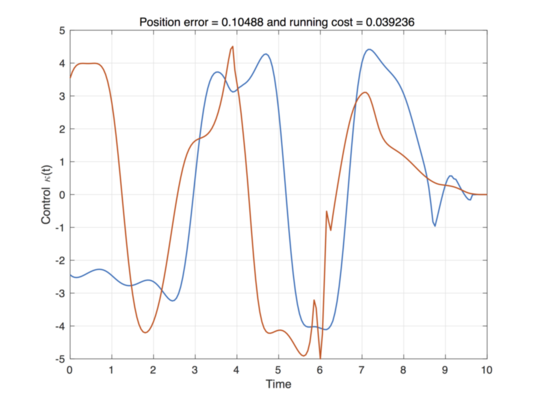
Then, one can get the following trajectories and optimal control solution.
subplot(1,2,2)
plot(tline,kappa','LineWidth',1.3);
xlabel('Time')
ylabel('Control \kappa(t)')
title(['Total Time = ',num2str(tline(end)),' and running cost = ',num2str(Running_cost)])
grid on