Download Code
Define vector fields of ODE : Kuramoto control problem whose dynamics is
where we control the first oscillator,
in order to change the limit phase value to be 0.
We first define the system of ODEs in terms of symbolic variables.
clear all
clc

m = 10;  %% [m]: number of oscillators, which we may change later.

th = sym('th', [m,1]);  %% [th_i]: phases of oscillators, $\theta_i$
om = sym('om', [m,1]);  %% [om_i]: natural frequencies of osc., $\omega_i$
KK = sym('K',[m,m]); %% [Ki_j]: the coupling network matrix, $K_{i,j}$

syms Nsys;   %% [Nsys]: the vector fields of ODEs
thth = repmat(th,[1 m]);
Nsys = om + (1./m)*sum(KK.*sin(thth.' - thth),2);   %% Kuramoto interaction terms
syms u; %% [u]: One-dimensional control term
Nsys(1) = Nsys(1) + u;    %% For the first particle, we put the control term


%% latex(Nsys)
The system is as follows:

Linearized model and numerical data setting
We now construct the linearized system using Jacobian:
syms F; %% [F]: The system without control
F = subs(Nsys,u,0);

syms Amat Bmat; %% [Amat, Bmat]: Symbolic versions of the matrix A and B
th_eq = zeros(m,1); %% Evaluation of Jacobian is at equilibrium, [0;0;0;0].
Amat = subs(jacobian(F,th),th,th_eq);
Bmat = diff(subs(Nsys,th,th_eq),u);
Construction of numerical matrices $A$ and $B$:
We next set the physical parameters. Natural frequencies, however, we put them zero to apply linear-quadratic control model.
The coupling network matrix is set to be random near ones(m,m):
KK_init = ones(m,m)+0.2*(2*(rand(m,m)-0.5));
and save it in the folder ‘functions/coupling.mat’.
om_init = zeros(m,1);
load('functions/coupling.mat','KK_init');

A = double(subs(Amat,[om,KK],[om_init,KK_init]));
B = double(subs(Bmat,[om,KK],[om_init,KK_init]));
Construction of the LQR controller and its evaluation
We design the LQR controller and solve it with linearized model.
The cost is only for the symmetric quadrature at $[0,0,0]$ since we want all of them to be 0.
R = 1; Q = diag(ones(m,1));
[ricsol,cleig,K,report] = care(A,B,Q);
K %% Present the feedback matrix
K =

  Columns 1 through 7

    0.6358    0.2930    0.2924    0.2829    0.2604    0.3013    0.2775

  Columns 8 through 10

    0.2777    0.2701    0.2713
Practically, any $K$ with positive elements can make the limit point to be 0, e.g., K=[1,1,1].
The initial condition is chosen on $[-0.55\pi,0.55\pi]$ by
ini = 0.55*pi()*(2*(rand(m,1)-0.5));
which is stored in the functions folder, ‘functions/ini.mat’.
load('functions/ini.mat','ini'); %% Safe data

tspan = [0,10];
1) Simulate the nonlinear dynamics without any control: $u = 0$.
syms Isys_ori;
Isys_ori = subs(F,[om,KK],[om_init,KK_init]);
Isys_ori_ftn_temp = matlabFunction(Isys_ori,'Vars',{th});
Isys_ori_ftn = @(t,x) Isys_ori_ftn_temp(x);

[timenc, statenc] = ode45(Isys_ori_ftn,tspan, ini); %% Solve ODE with 'ode45'
2) Simulate the linear dynamics with CARE function
f_ctr = @(x) -K*x;

i_linear = @(t,x) A*x + B*f_ctr(x);

[time, state] = ode45(i_linear,tspan, ini);
3) Simulate the nonlinear dynamics with the same control
syms Isys;
Isys = subs(Nsys,[om,KK,u],[om_init,KK_init,(-K*th)]);
Isys_ftn_temp = matlabFunction(Isys,'Vars',{th});
Isys_ftn = @(t,x) Isys_ftn_temp(x);

[timen, staten] = ode45(Isys_ftn,tspan, ini);
Visualization
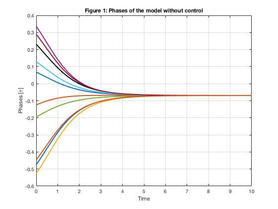
plot(timenc, statenc(:,1)/pi(),'-k','LineWidth',2) %% The first oscillator is black-colored.
hold on
plot(timenc, statenc(:,2:m)/pi(),'LineWidth',2)
grid on
xlabel('Time')
ylabel('Phases [\pi]') %% The unit is $\pi$.
title('Figure 1: Phases of the model without control')
hold off
clf
plot(time, state(:,1)/pi(),'-k','LineWidth',2)
hold on
plot(time, state(:,2:m)/pi(),'LineWidth',2)
grid on
xlabel('Time')
ylabel('Phases [\pi]')
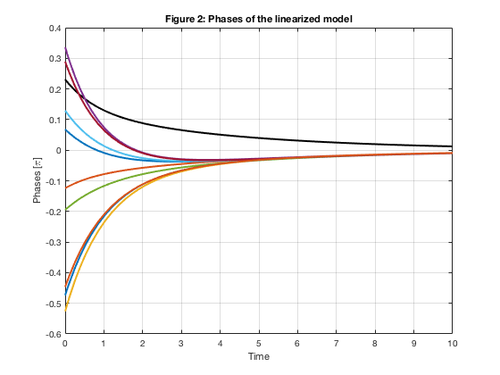
title('Figure 2: Phases of the linearized model')
hold off
clf
plot(timen, staten(:,1)/pi(),'-k','LineWidth',2)
hold on
plot(timen, staten(:,2:m)/pi(),'LineWidth',2)
grid on
xlabel('Time')
ylabel('Phases [\pi]')
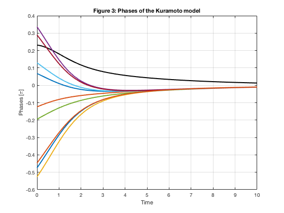
title('Figure 3: Phases of the Kuramoto model')
hold off
In Figure 1, the limit point is not zero since the mean value of initial phases is nonzero.
Figure 2 shows that the first oscillator keeps it phase above zero to make the final phases zero.
The nonlinear model has less decay then the linearized model, but goes to zero in Figure 3.
Failure of LQR control for large initial data
The initial data is from
ini2 = pi()*(2*(rand(m,1)-0.5));
which is uniformly distributed on $[-\pi,\pi]$. We expect the limit point to be separated in the real line with differences $2\pi$.
load('functions/ini2.mat','ini2'); %% Separated data

f_ctr = @(x) -K*x;

i_linear = @(t,x) A*x + B*f_ctr(x);

tspan = [0,20];
[time, state] = ode45(i_linear,tspan, ini2);

syms Isys;
Isys = subs(Nsys,[om,KK,u],[om_init,KK_init,(-K*th)]);
Isys_ftn_temp = matlabFunction(Isys,'Vars',{th});
Isys_ftn = @(t,x) Isys_ftn_temp(x);
[timen, staten] = ode45(Isys_ftn,tspan, ini2);

figure(4)
plot(time, state(:,1)/pi(),'-k','LineWidth',2)
hold on
plot(time, state(:,2:m)/pi(),'LineWidth',2)
grid on
xlabel('Time')
ylabel('Phases [\pi]')
title('Figure 4: Phases of the linearized model')
hold off

figure(5)
plot(timen, staten(:,1)/pi(),'-k','LineWidth',2)
hold on
plot(timen, staten(:,2:m)/pi(),'LineWidth',2)
grid on
xlabel('Time')
ylabel('Phases [\pi]')
title('Figure 5: Phases of the Kuramoto model')
hold off
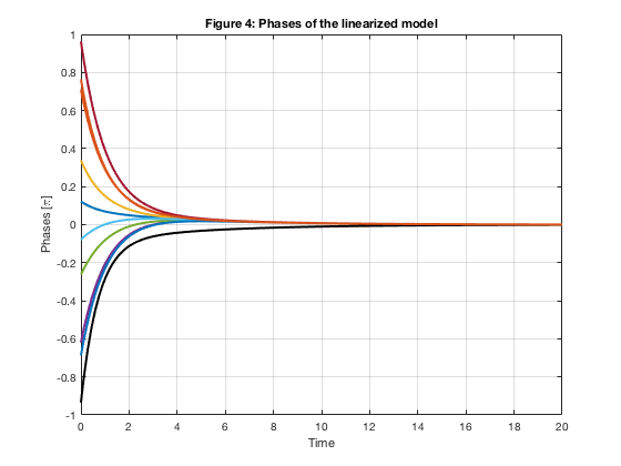
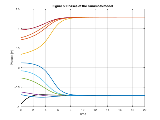
We can see that $\theta_1$ does not tend to zero in Figure 5 since $K\times\Theta$ is near zero already. Linear feedback control is not enough, or too weak, for this setting.