Download Code
Summary of example objective The goal of this tutorial is to use LQR theory applied to a model of collective behavior. The model choosen shares a formal structure with the semidiscretization of the semilinear 1d heat equation.
Consider $N$ agents $y_i$ for $i=1,…,N$, and let $y=(y_1,…,y_N)\in \mathbb{R}^N$.
The model considered is the following:
where $A$ is a matrix of the form:
and $\vec{G}:\mathbb{R}^N\to\mathbb{R}^N$ is a non linear function of the form
where $G$ is a non-linear function, matrix $A$ models the interaction between agents. Agent $i$ changes its state according to the state of agent $i+1$ and $i-1$ in a linear way plus a non-linear effect that depends only on his state.
Note that the manifold
is invariant under $F$. Indeed, taking $x\in\mathcal{M}_N$ we have that
Therefore, the mean will follow the following 1-d dynamical system
Here we will consider that $G(0)=0$ and that $DG(0)>0$, we have an unstable critical point at 0. Let N=20,
N=2;
A=full(gallery('tridiag',N,1,-2,1));
A(1,1)=-1;
A(N,N)=-1;
and that
here $G$ is taken in the following form (and we compute also its derivative).
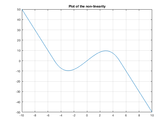
The non-linearity choosen is:
a=5;
c=0.20;
syms G(x);
syms DG(x);
G(x) = piecewise(x<=-a, -2*a*a*x*c-2*a*a*a*c, a<=x, -2*a*a*x*c+2*a*a*a*c, -a<x<a, -c*x*(x-a)*(x+a));
DG(x) = diff(G,x);
G=@(x)double(G(x));
DG = @(x)double(DG(x));

close all
figure(1)
fplot(G,[-10,10])
title('Plot of the non-linearity')
hold off
grid
The function field assigns an $N$ dimensional vector corresponding to the field for every point in $\mathbb{R}^N$, matrix $A$ and the nonlinear function $G$
F =

  function_handle with value:

    @(t,y)field(A,G,y)
Now its the turn to define our cost functional. Our goal will be to stabilize the system in a critical point inside the manifold $\mathcal{M}_N$. Notice that, in particular $0$ is a critical point.
We will choose the matrix $Q$ in a way that the vector that defines $\mathcal{M}_N$ is an eigenvector of the matrix $Q$, we have seen that the manifold $\mathcal{M}_N$ is invariant under the flow. Our cost functional will take into account if we are not in this manifold.
We check that its eigenvalues are non-negative
Q=eye(N)-ones([N N])/N;
EigQ=eig(Q)
And we define $R$ being just the identity
Linearize arround the unstable equilibrium 0 and obtain the linearized system $\dot{y}=Ly$
we set our control matrix B
One has to check the rank of the controllability matrix to see if we satisfy the Kalman rank condition
Co=ctrb(L,B);
rank=rank(Co)
Once it is done, we are in the position of solving the algebraic Riccati equation
[ricsol,cleig,K,report] = care(L,B,Q);
Consider a time span and an initial datum
radius = 6
ini    = radius*(-0.5+rand(N,1))
radius =

     6


ini =

   -1.3855
    1.4941
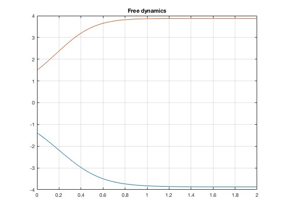
the free dynamics would result
tspan = [0, 2];
[t,y] = ode45( F, tspan, ini);

figure(2)
for i=1:N-1
    plot(t, y(:,i));
    hold on;
end
plot(t, y(:,N))
title('Free dynamics')
hold off
grid
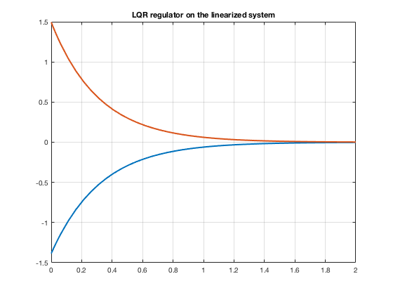
Now the LQ controller with the linear and the non-linear dynamics
u_lq = @(t,x) -K * x;


i_linear = @(t,x) L*x + B*u_lq(t,x);
[time, state] = ode45(i_linear,tspan, ini);

i_nonlinear = @(t,x)[F(t,x)+B*u_lq(t,x)];
[timen, staten] = ode45(i_nonlinear,tspan, ini);

figure(3)
for i=1:N-1
    plot(time, state(:,i),'LineWidth',2);
    hold on;
end
plot(time, state(:,N),'LineWidth',2)
grid on
title('LQR regulator on the linearized system')
hold off
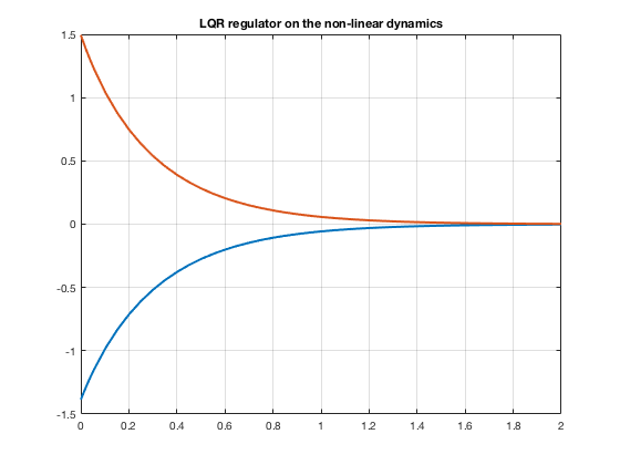
[timen, staten] = ode45(i_nonlinear,tspan, ini);

figure(4)
for i=1:N-1
    plot(timen, staten(:,i),'LineWidth',2);
    hold on;
end
plot(timen, staten(:,N),'LineWidth',2)
grid on
title('LQR regulator on the non-linear dynamics')
hold off