Download Code
1 Introduction
We are interested in the numerical discretization of the Kolmogorov equation [12]
where $\mu>0$ is a diffusive function and $v$ a potential function.
This is one example of degenerate advection-diffusion equations which have the property of hypo-ellipticity (see for instance, [6, 13, 14]), ensuring the $C^\infty$ regularity of solutions for $t>0$ ([6]).
In the present case, the generator of the semigroup is constituted by the superposition of operators $\mu \partial_{xx}$ and $ v(x) \partial_y $. Despite the presence of a first order term, that could lead to transport phenomena and, consequently, to the lack of smoothing, the regularizing effect is ensured by the fact that the commutator of these two operators is non-trivial, allowing to gain regularity in the variable $y$. A full characterization of hypo-ellipticity can be found in [6].
Solutions of (1) experience also decay properties as $t\to \infty$. This is also a manifestation of hypo-coercivity (in the sense developed by Villani [13], [14]) as a byproduct of the hidden interaction of the two operators entering in the generator of the semigroup.
In this particular case $\mu=1$ and $v(x)=x$, using the Fourier transform, the fundamental solution of (1) (starting from an initial Dirac mass $\delta_{(x_0, y_0)}$) can be computed explicitly getting the following anisotropic Gaussian kernel
which exhibits different diffusivity and decay scales in the variables $x$ and $y$.
In view of the structure of the fundamental solution, one can deduce the following decay rates:
for solutions with initial data $f_0$ in $L^2$. Similar decay properties can be predicted by scaling arguments, due to the invariance properties of the equation in (\ref{kolmo}).
These decay properties are of anisotropic nature and of a different rate in the $x$ and $y$-directions. Indeed, in the $x$-direction, as in the classical heat equation, we observe a decay rate of the order of $t^{-1/2}$, while, in the $y$-variable, the decay is of order $t^{-3/2}$.
The obtention of these decay properties by energy methods has been a challenging topic of particular interest when dealing with more general convection-diffusion models that do not allow the explicit computation of the kernel. In this effort, the asymptotic behavior of Kolmogorov equation and several other relevant kinetic models was investigated intensively through the concept and techniques of hypo-coercivity, which allow to make explicit the hidden diffusivity and dissipativity of the involved operators (see [13], [14] and the previous references therein).
The literature on the asymptotic behaviour of models related with Kolmogorov equation is huge. We refer for instance to [8], [9], [2] for earlier works, and to [4], [5] for more recent approaches. Roughly speaking, it is by now well known that, constructing well-adapted Lyapunov functionals through variations of the natural energy of the system, one can make the dissipativity properties of the semigroup emerge and then obtain the sharp decay rates. These techniques have been developed also in other contexts such as partially dissipative hyperbolic systems (see [1]).
In [10] Porretta and Zuazua introduces a numerical scheme that preserves this hypo-coercivity property at the numerical level, uniformly on the mesh-size parameters. The issue is relevant from a computational point of view since, as it has been observed in a number of contexts (wave propagation, dispersivity of Schrödinger equations, conservation laws, etc. [15], [7]), the convergence property in the classical sense of numerical analysis (a property that concerns finite-time horizons) is not sufficient to ensure the asymptotic behavior of the PDE solutions to be captured correctly. The fact that the numerical approximation schemes preserve the decay properties of continuous solutions can be considered as a manifestation of the property of numerical hypo-coercivity.
In [3] Foster et al introduces a numerical scheme which preserves the long time behavior of solutions to the Kolmogorov equation. The method presented is based on a self-similar change of variables technique to transform the Kolmogorov equation into a new form, such that the problem of designing structure preserving schemes, for the original equation, amounts to building a standard scheme for the transformed equation. We also present an analysis for the operator splitting technique for the self-similar method and numerical results for the described scheme.
Here, instead of, we investigate this behavior using the characteristics-Galerkin finite element method (trough Freefem++ [11]) and in particular, we confront the results to those obtained in [3].
2 Description of the numerical scheme
At the numerical level, we employ a finite element method based on characteristics-Galerkin technique, and for the sake of simplicity and ease, we use the Freefem ++ software ([11]). As described above, solution of Equation (1) does not only diffuses in the direction of x, by the effect of the diffusion operator $\partial_{xx} f$, but it is also diffuses in the direction of $y$, due to the transport equation $\partial_t f - v(x) \partial_y f$. We will treat both effects, transport and diffusion separately, using the characteristics method, that we recall hereafter, for the equation $\partial_t f - v(x) \partial_y f$ and linear or quadratic finite element to discretise the diffusion term.
2.1 Transport
Let us consider the following scalar two dimensional transport equation
for some function $g$. Let (x,y,t)$\in \mathbb{R}^2 \times \mathbb{R}^+$. This transport equation can be written using the total derivative
if and only if the curve $( X_{x,y,t}(s),s)$ satisfies the system of ordinary differential equation
Under suitable assumptions on $ c$, the problem is well defined and there exists a unique solution to (6) $ X_{x,y,t}$, called the characteristic curve reaching (or passing from) the point $(x,y)$ at time $t$.
Since we cannot compute explicitly, in general, the solution of the equation (6), hence (4), we look for an approximate solution. Noting $\delta t>0$ the time step and $t_{n+1} = t_n + \delta t$, an easy manner to approximate the solution of Equation (4) is to perform a backward convection by the method of characteristic
where $f^n(x,y) = f(x,y,t_n)$ and $ X_{x,y,t_n}(x)$ is an approximation, as shown below, of the solution at time $t_n=n \delta t$ of the ordinary differential equation (6) for $s\in(t_n,t_{n+1})$ with the final data $ X_{x,y,t}(t_{n+1}) = (x,y)$.
Assuming $f$ regular enough, by Taylor expansion, one can write
Applying also a Taylor expansion to the function $t\mapsto f^n((x,y)-t c( X_{x,y,t_n}(t_n),t_n))$, we get
and therefore one can approximate $f^n( X_{x,y,t}(t_{n}))$ by $f^n((x,y)- \delta t \ c( X_{x,y,t_n}(t_n),t_n))$. For the sake of clarity, in the sequel, we note $X(t)$ the characteristic curve passing through the point $(x,y)$ at time $t$.
2.2 Numerical algorithm
For numerical purpose, we consider Equation (1) in $\Omega \subset \mathbb{R}^2$ with homogeneous Neumann boundary conditions. Keeping in mind the characteristic method, Equation (1) can be written
where $ n$ stands for the outward unit normal to $\Omega$, and for all $s\in(0,t)$, $ X$ is the solution of
Here, we use the following notations
Formally, thus, one can write, for any $\varphi \in V$ for some functional space, the weak form of Equation (8) as follows
Let us denote $t_0<t_1<\ldots < t_M = T$ be the discrete time with $t_n = n \delta t$ where $\delta t$ denotes the time step. We set $M = T/\delta t$.
Using the method of characteristic for the total derivative (see section 2.1), the weak form (10) can be approximated by
or
where
Here $(\cdot,\cdot)$ is the inner product in $L^2(\Omega)$.
Therefore, denoting $\tau_h$ a partition of $\Omega$ by triangles and $V_h$ the $P_k$-finite element space (of degree $k$),
the weak discrete form of the problem (8) is
Find ${f_h^n}_{n=1}^{M=T/\delta t} \subset V_h$ such that for $n=1,\dots, M$,
The Freefem++ script corresponding to the problem may as follows
</ol>
Freefem++ CODE:
- Freefem++ code for prog_control.m:
/*
C****************************************************************************C
C                                                                            C
C     This program solve the Kolmogorov equation                             C
C     f_t-mu*f_{xx}-v(x) f_y = 0 on Omega x [0,T]                            C
C     with free boundary conditions                                          C
C     using the Characteristic-Galerkin Finite Element Method                C
C********************************************C*******************************C
C     f(i,j)   ==> unknown scalar function   C
C     phi(i,j) ==> test function             C
C     v(i)     ==> scalar potential function C
C********************************************C
*/

//Omega : square mesh [0,20]x[0,20]
real aa = 10;
real x0=-aa,x1=aa;
real y0=-aa,y1=aa;
int m = 100;
mesh Th=square(m,m,[x0+(x1-x0)*x,y0+(y1-y0)*y]);


real Tf  = 10,
     dt  = 0.01,
     mu  = 1;    // viscosity parameter (see equation above)


fespace Vh(Th,P2);     // P1 linear finite element
Vh f0 = exp(-x^2-y^2), // initial data
   phi,                // test function
   v=-x,
   f;


for(real t=0;t<=Tf;t=t+dt)
{
  Vh c=convect([0,v(x,y)],-dt,f0);
  solve Kolmogorov(f,phi)
            =
              int2d(Th)(f*phi/dt +mu*(dx(f)*dx(phi)))
    	    - int2d(Th)(c/dt*phi)
	    ;
  f0=f;
}
3 Numerical experiment
In this section we present a test case, [3], for which we confront to an exact solution of the Kolmogorov Equation (1) with $\mu=1$ and $v(x)=x$. In particular, we compare our results to the one obtained in [3]. For our numerical test case, we have used linear finite element.
The initial value problem (1) with the initial data $f_0(x,y) = \exp(-x^2-y^2)$ admits the following exact solution
$$f_{ex}(x,y,t) = \frac{\exp\left(-\frac{(( 3+3t^2 +4t^3)x^2 +6t(1+2t)xy+3(1+4t)y^2)}{(3+12t+4t^3 +4t^4)}\right)}{\sqrt{1 + 4 t + 4/3 t^2 + 4/3 t^4}} \ . $$
As done in [3], for each numerical tests, we have considered the time interval, and problem domain to be respectively $[0, T=10]$ and $\Omega = [−10, 10] \times [−10,10]$, The time step is kept constant equal to $\delta t = 0.01$ and the number of triangles along each side of the domain is given by $m=50$, $100$ and $150$.
As one can see in the video above, the support for the function grows beyond the problem domain in the given time interval and interact with boundary conditions. This interaction, since we do not use here transparent boundary conditions, increases the error as one can also observe in Figure 1. We also show the time evolution of $\|f(\cdot,t)-f_{ex}(\cdot,t)\|_2$, $\|\partial_xf(\cdot,t)\|_2$, $\|\partial_y f(\cdot,t)\|_2$ and
$$D(t)=\left(\| f(t)\|_{L^2}+ \sqrt t\, \| \partial_x f(t) \|_{L^2}+ t^{\frac 32} \|\partial_y f(t)\| _{L^2}\right)/||f_0||_{L^2} \ ,$$ in Figure 2. The $L_2$ error at time time $T=10$ is approximately $0.0072$ as one can see in Figure 2(a). Moreover, the error $\int_0^T \| f(\cdot,t)-f_{ex}(\cdot,t)\|_2 dt $ is approximately of order $0.02$. We also observe, due to the interaction with the boundary conditions that the errors increase sensibly for each numerical experiments approximately at time $t\approx 8.5$. Therefore, in order to compute the numerical order of convergence, we have computed for each $m$, $m\mapsto \max_t\left( \|f(\cdot,t)-f_{ex}(\cdot,t)\|_2\right)$. We find almost the order $1$ which is satisfactory. Finally, we have computed the quantity
$$D(t) =\left(\| f(t)\|_{L^2}+ \sqrt t\, \| \partial_x f(t) \|_{L^2}+ t^{\frac 32} \|\partial_y f(t)\| _{L^2}\right)/||f_0||_{L^2}\ , $$
for which we numerically show that the constant for the decay rates is $C=1$ as shown in Figure 2(d)
Movie 1: Numerical simulation of the test case .
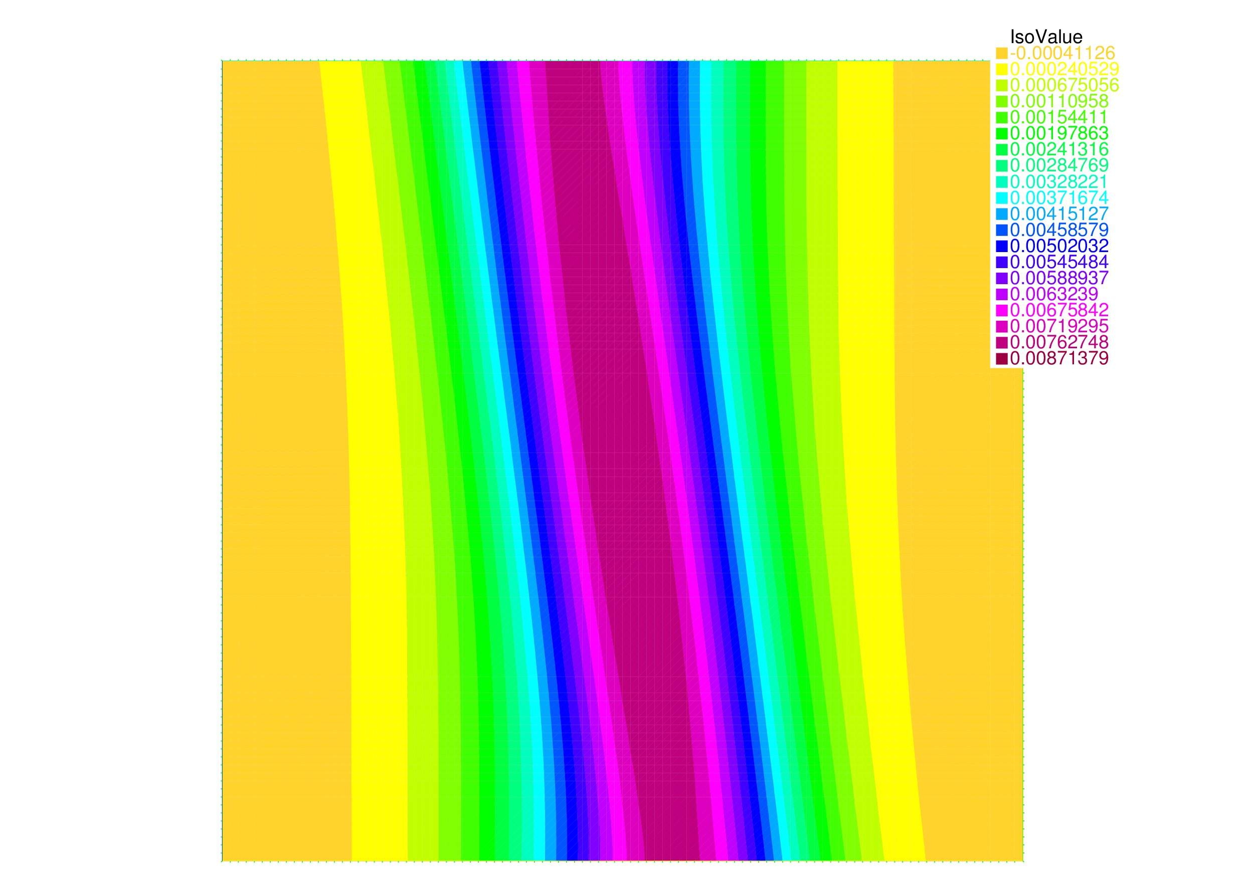 Figure 1.a: Numerical and exact solution at time $T=10$, Freefem solution with $m=100$
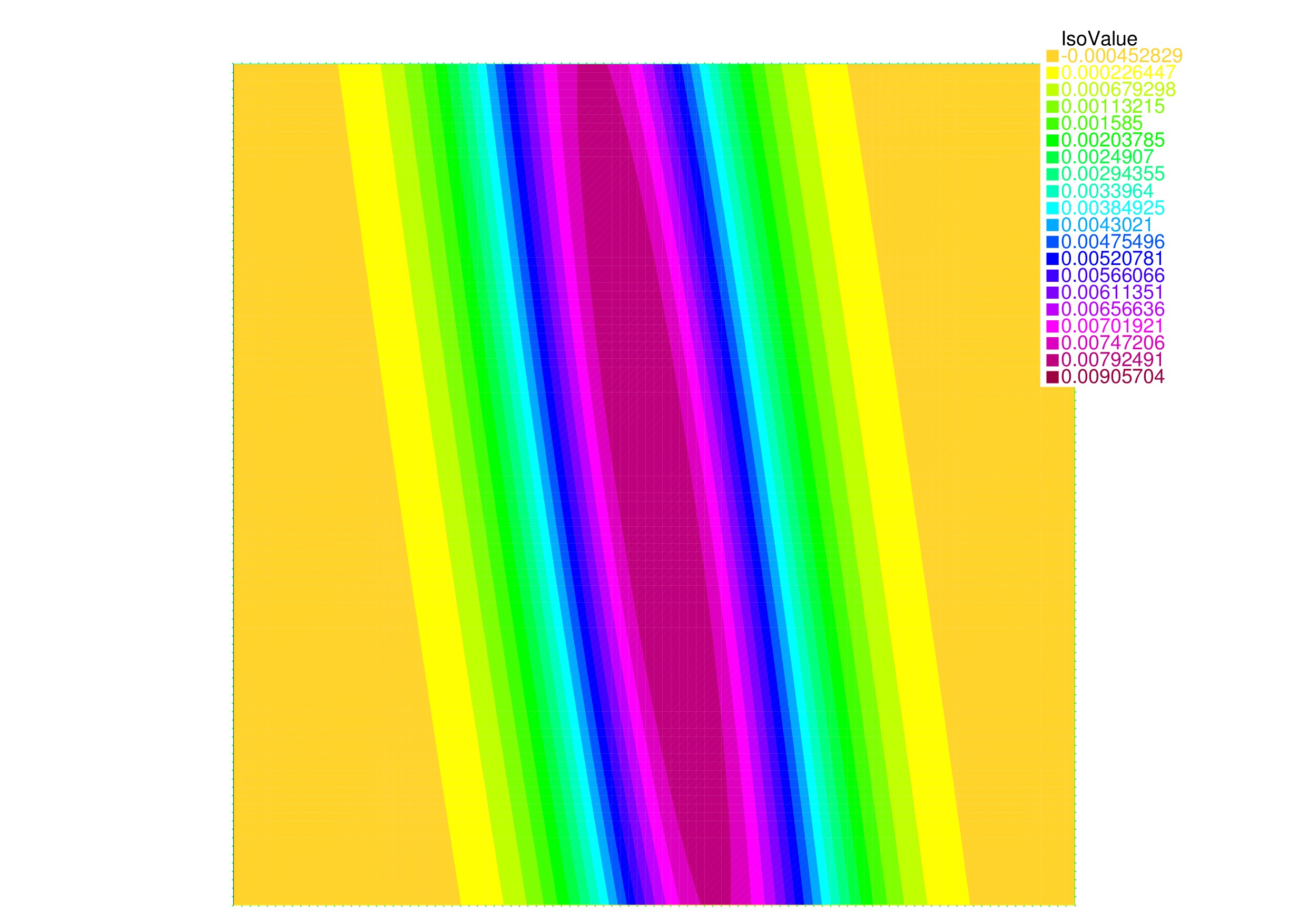 Figure 1.b: Numerical and exact solution at time $T=10$, Exact solution
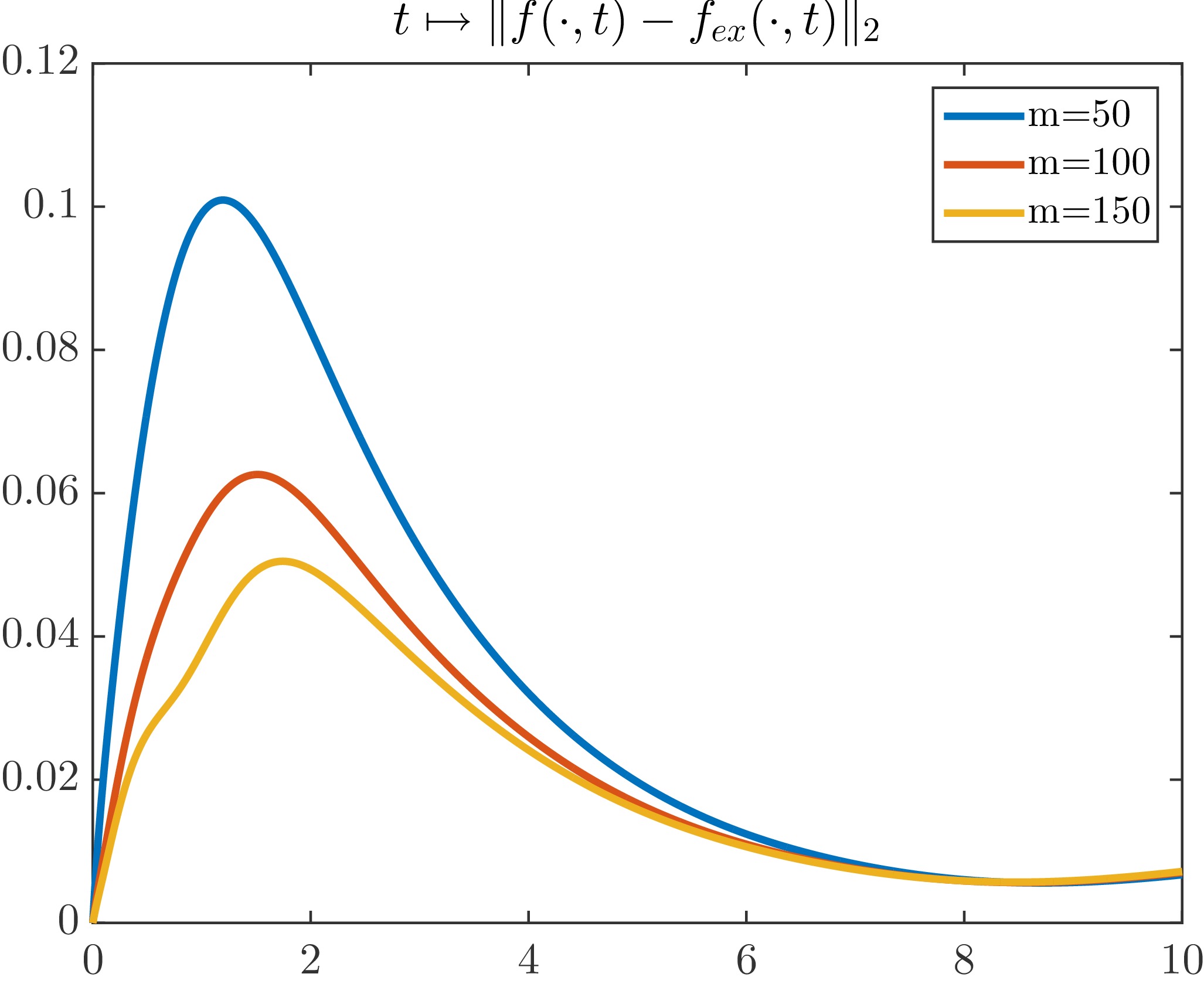 Figure 2.a: $L_2$ errors, $t\mapsto\|f(\cdot,t)-f_{ex}(\cdot,t)\|_2$
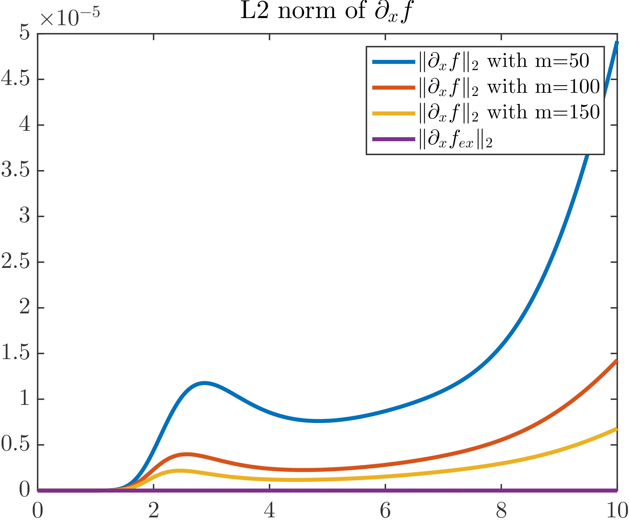 Figure 2.b: $L_2$ errors, $t\mapsto \|\partial_xf(\cdot,t)\|_2$
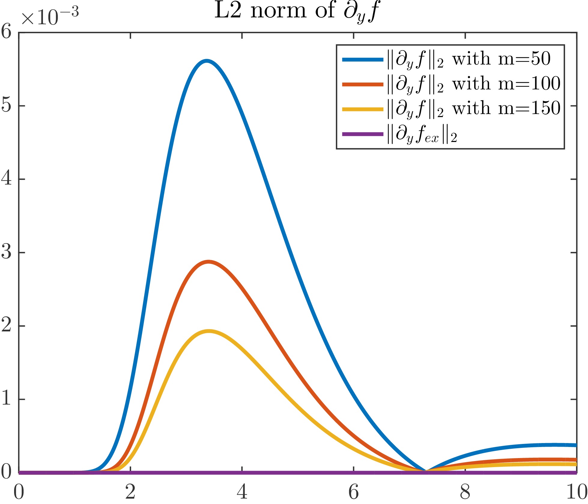 Figure 2.c: $L_2$ errors, $t\mapsto \|\partial_yf(\cdot,t)\|_2$
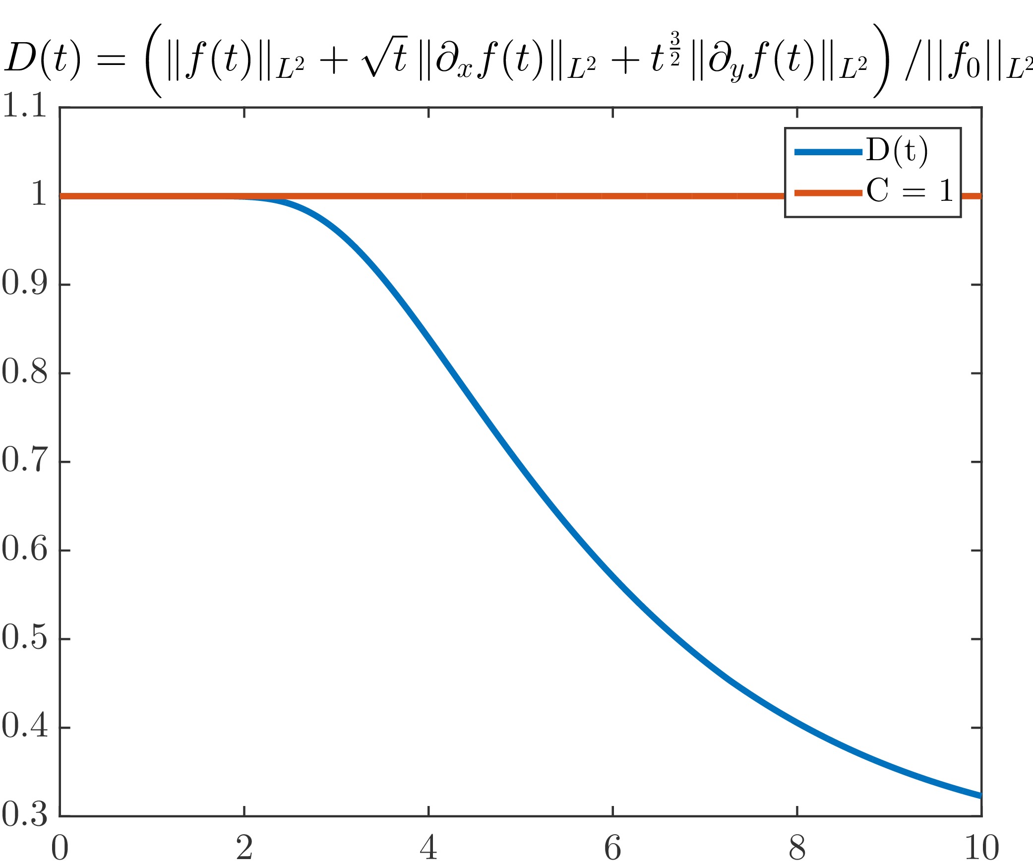 Figure 2.d: $L_2$ errors,$t\mapsto D(t)$
To end, we present a last numerical simulation of rotating and moving initial data.
Movie 2: Numerical simulation on $\Omega = [0,10]\times[0,20]$, $[0,T=0.6]$ with $\mu=10^{-3}$, $v(x)=-x$ and $f_0(x,y) = 20 \exp(-(y-15)^2) \exp(-0.1(x-10)^2)$.
Figure 2.d: $L_2$ errors,$t\mapsto D(t)$
To end, we present a last numerical simulation of rotating and moving initial data.
Movie 2: Numerical simulation on $\Omega = [0,10]\times[0,20]$, $[0,T=0.6]$ with $\mu=10^{-3}$, $v(x)=-x$ and $f_0(x,y) = 20 \exp(-(y-15)^2) \exp(-0.1(x-10)^2)$.
Bibliography
[1] K. Beauchard and E. Zuazua, Sharp large time asymptotics for partially dissipative hyperbolic systems, Arch. Ration. Mech. Anal. 199 (2011) 177-7227.
[2] A. Carpio, Long-time behavior for solutions of the Vlasov-Poisson-Fokker-Planck equation, Mathematical methods in the applied sciences 21 (1998), 985-1014.
[3] E. L. Foster, J. Lohéac and M.-B. Tran, A Structure Preserving Scheme for the Kolmogorov Equation, preprint 2014 (arXiv:1411.1019v3).
[4] F. Hérau, Short and long time behavior of the Fokker-Planck equation in a confining potential and applications, J. Funct. Anal. 244 (2007), 95-118.
[5] F. Hérau and F. Nier, Isotropic hypoellipticity and trend to equilibrium for the Fokker-Planck equation with a high-degree potential, Arch. Ration. Mech. Anal. 171 (2004), 151-218.
[6] L. Höormander, Hypoelliptic second order differential equations, Acta Math. 119 (1967), 147-171.
[7] L. Ignat, A. Pozo and E. Zuazua, Large-time asymptotics, vanishing viscosity and numerics for 1-D scalar conservation laws, Math of Computation, to appear.
[8] A. M. Il'in, On a class of ultraparabolic equations, Soviet Math. Dokl. 5 (1964), 1673-1676.
[9] A. M. Il'in and R. Z. Kasminsky, On the equations of Brownian motion, Theory Probab. Appl. 9 (1964), 421-444.
[10] A. Porretta and E. Zuazua, Numerical hypocoercivity for the Kolmogorov equation, Mathematics of Computation 86.303 (2017): 97-119.
[11] Frédéric Hecht, Olivier Pironneau, A~Le~Hyaric and K~Ohtsuka, Freefem++ manual, 2005.
[12] A. Kolmogoroff, Zufallige bewegungen (zur theorie der brownschen bewegung) Annals of Mathematics, pages 116--117, 1934.
[13] C. Villani, Hypocoercivity, Mem. Amer. Math. Soc. 202 (2009).
[14] C. Villani, Hypocoercive diffusion operators, In International Congress of Mathematicians, Vol. III, 473-498. Eur. Math. Soc. Zürich, 2006.
[15] E. Zuazua, Propagation, observation, and control of waves approximated by finite difference methods, SIAM Review, 47 (2) (2005), 197-243.