Download Code
Shows the propagation of the solution of a fractional Schrodinger equation with concentrated and highly oscillatory initial datum. The solution remains concentrated along the rays of geometric optics
N = 250;
L = 1;
hx = (2*L)/(N+1);
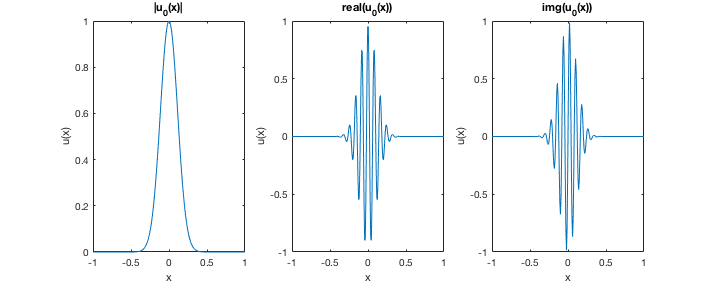
Definition of the initial datum u0 as a function_handle. u0 is chosen as a Gaussian profile multiplied by a higly oscillatory function
x0 = 0; %% Center of the Gaussian profile
gamma = hx^(-0.9); %% Amplitude of the Gaussian profile
fr = (1/hx)*pi^2/16; %% Frequency of the oscillations
u0 = @(x) exp(-0.5*gamma*(x-x0).^2).*exp(1i*fr*x);
Plot of the initial datum
fig = gcf;
set(gcf,'Units','pixels','Position',[427 306 712 284])

x = -L:hx:L;

subplot(1,3,1) %% Modulus
plot(x,abs(u0(x)))
title('\vertu_0(x)\vert')
xlabel('x'); ylabel('u(x)');

subplot(1,3,2) %% Real part
plot(x,real(u0(x)))
title('real(u_0(x))')
xlabel('x'); ylabel('u(x)');

subplot(1,3,3) %% Imaginary part
plot(x,imag(u0(x)))
title('img(u_0(x))')
xlabel('x'); ylabel('u(x)');
Solution for s = 1/2
Define the characteristic parameters of the problem
s = 0.5  %% Order of the fractional Laplacian
L        %% Extrema of the space interval
N        %% Number of points in the space mesh
T = 5    %% Length of the time interval
u0       %% The function_handle that we have showed before.
s =

    0.5000


L =

     1


N =

   250


T =

     5


u0 =

  function_handle with value:

    @(x)exp(-0.5*gamma*(x-x0).^2).*exp(1i*fr*x)
To solve the equation, we call the function fractional_schr. The solution of the equation is stored in the u variable.
[x,t,u] = fractional_schr(s,L,N,T,u0);
Now we can see a graphical interpretation
[X,T] = meshgrid(x,t);
%%
clf
mesh(X,T,u');
view(0,90)
xlabel('x'); ylabel('t'); title('Ray Evolution');
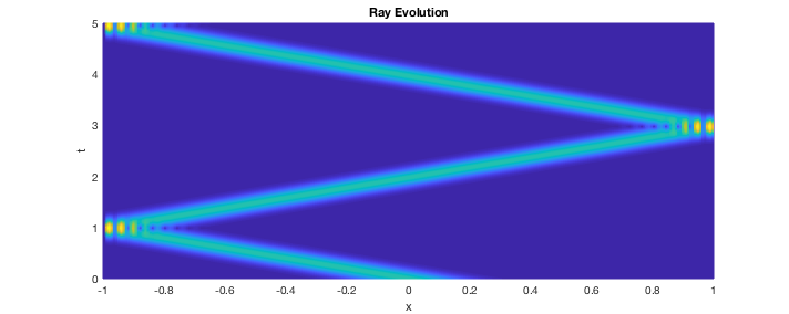
By typing “animation(x,t,u)” in the MATLAB console you can see the evolution in time of this wave.